Chapter 7 Pumps and how they operate in a hydraulic system
For any system delivering water through circular pipes with the assistance of a pump, the selection of the pump requires a consideration of both the pump characteristics and the energy required to deliver different flow rates through the system. These are described by the system and pump characteristic curves. Where they intersect defines the operating point, the flow and (energy) head at which the pump would operate in that system.
7.1 Defining the system curve
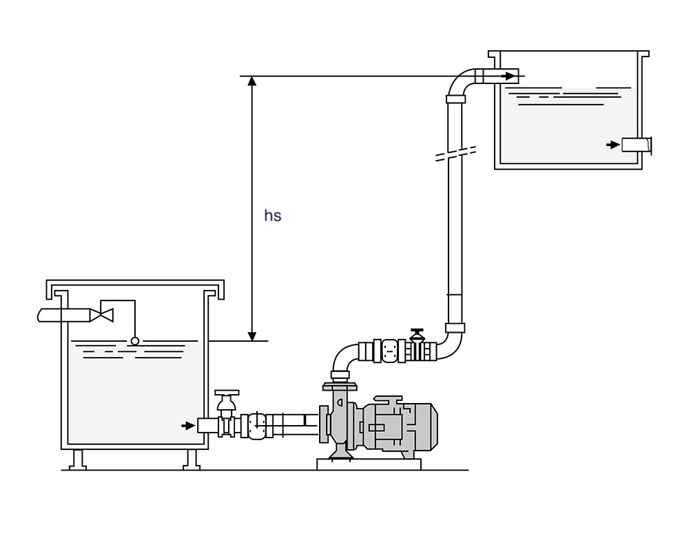
Figure 7.1: A simple hydraulic system (from https://www.castlepumps.com)
For a simple system the loss of head (energy per unit weight) due to friction, \(h_f\), is described by the Darcy-Weisbach equation, which can be simplified as in Equation (7.1). \[\begin{equation} h_f = \frac{fL}{D}\frac{V^2}{2g} = \frac{8fL}{\pi^{2}gD^{5}}Q^{2} = KQ{^2} \tag{7.1} \end{equation}\]
The total dynamic head the system requires a pump to provide, \(h_p\), is found by solving the energy equation from the upstream reservoir (point 1) to the downstream reservoir (point 2), as in Equation (7.2). \[\begin{equation} h_p = \left(z+\frac{P}{\gamma}+\frac{V^2}{2g}\right)_2 - \left(z+\frac{P}{\gamma}+\frac{V^2}{2g}\right)_1+h_f \tag{7.2} \end{equation}\]
For the simple system in Figure 7.1, the velocity can be considered negligible in both reservoirs 1 and 2, and the pressures at both reservoirs is atmospheric, so the Equation (7.2) can be simplified to (7.3). \[\begin{equation} h_p = \left(z_2 - z_1\right) + h_f=h_s+h_f=h_s+KQ^2 \tag{7.3} \end{equation}\]
Using the hydraulics package, the coefficient, K, can be calculated manually or using other package functions for friction loss in a pipe system using \(Q=1\). Using this to develop a system curve is demonstrated in Example 7.1.
Example 7.1 Develop a system curve for a pipe with a diameter of 20 inches, length of 3884 ft, and absolute roughness of 0.0005 ft. Use kinematic viscocity, \(\nu\) = 1.23 x 10⁻⁵ ft2/s. Assume a static head, z2 - z1 = 30 ft.
ans <- hydraulics::darcyweisbach(Q = 1,D = 20/12, L = 3884, ks = 0.0005, nu = 1.23e-5, units = "Eng")
cat(sprintf("Coefficient K: %.3f\n", ans$hf))
#> Coefficient K: 0.160
scurve <- hydraulics::systemcurve(hs = 30, K = ans$hf, units = "Eng")
print(scurve$eqn)
#> [1] "h == 30 + 0.16*Q^2"
For this function of the hydraulics package, Q is either in ft\(^3\)/s or m\(^3\)/s, depending on whether Eng or SI is specified for units. Often data for flows in pumping systems are in other units such as gpm or liters/s, so unit conversions would need to be applied.
7.2 Defining the pump characteristic curve
The pump characteristic curve is based on data or graphs obtained from a pump manufacturer, such as that depicted in Figure 7.2.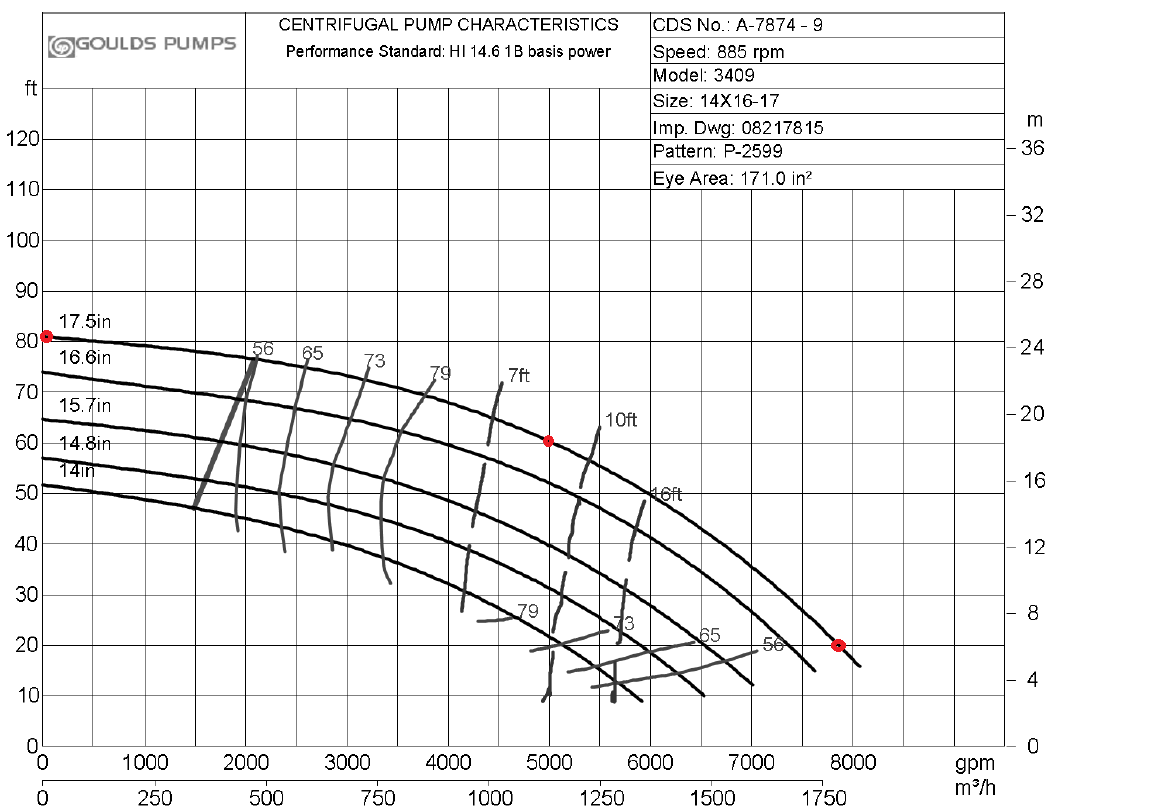
Figure 7.2: A sample set of pump curves (from https://www.gouldspumps.com). The three red dots are points selected to approximate the curve
The three selected points, selected manually across the range of the curve, are used to generate a polynomial fit to the curve. There are many forms of equations that could be used to fit these three points to a smooth, continuous curve. Three common ones are implemented in the hydraulics package, shown in Table 7.1.
| type | Equation |
|---|---|
| poly1 | \(h=a+{b}{Q}+{c}{Q}^2\) |
| poly2 | \(h=a+{c}{Q}^2\) |
| poly3 | \(h=h_{shutoff}+{c}{Q}^2\) |
The \(h_{shutoff}\) value is the pump head at \(Q={0}\).
Many methods can be used to fit a polynomial to a set of points. The hydraulics package includes the pumpcurve function for this purpose. The coordinates of the points can be input as numeric vectors, being careful to use correct units, consistent with those used for the system curve.
Manufacturer’s pump curves often use units for flow that are not what the hydraulics package needs, and the units package provides a convenient way to convert them as needed. Developing the pump characteristic curve using the hydraulics package is demonstrated in Example 7.2.
Example 7.2 Develop a pump characteristic curve for the pump in Figure 7.2, using the three points marked in red. Use the poly2 form from Table 7.1.
qgpm <- units::set_units(c(0, 5000, 7850), gallons/minute)
#Convert units to those needed for package, and consistent with system curve
qcfs <- units::set_units(qgpm, ft^3/s)
#Head units, read from the plot, are already in ft so setting units is not needed
hft <- c(81, 60, 20)
pcurve <- hydraulics::pumpcurve(Q = qcfs, h = hft, eq = "poly2", units = "Eng")
print(pcurve$eqn)
#> [1] "h == 82.5 - 0.201*Q^2"
The function pumpcurve returns a pumpcurve object that includes the polynomial fit equation and a simple plot to check the fit. This can be plotted as in Figure 7.3
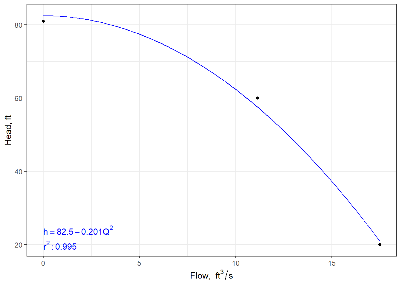
Figure 7.3: A pump characteristic curve
7.3 Finding the operating point
The two curves can be combined to find the operating point of the selected pump in the defined system. this can be done by plotting them manually, solving the equations simultaneously, or by using software. The hydraulics package finds the operating point using the system and pump curves defined earlier. Example 7.3 shown how this is done.
Example 7.3 Find the operating point for the pump and system curves developed in Examples 7.1 and 7.2.
oppt <- hydraulics::operpoint(pcurve = pcurve, scurve = scurve)
cat(sprintf("Operating Point: Q = %.3f, h = %.3f\n", oppt$Qop, oppt$hop))
#> Operating Point: Q = 12.051, h = 53.285
The function operpoint function returns an operpoint object that includes the a plot of both curves. This can be plotted as in Figure 7.4
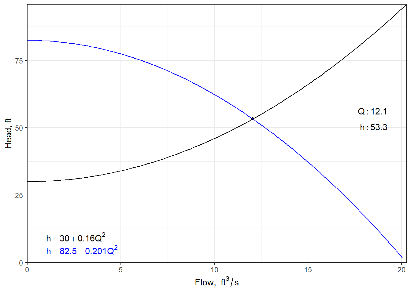
Figure 7.4: The pump operating point