Chapter 12 Management of water resources systems
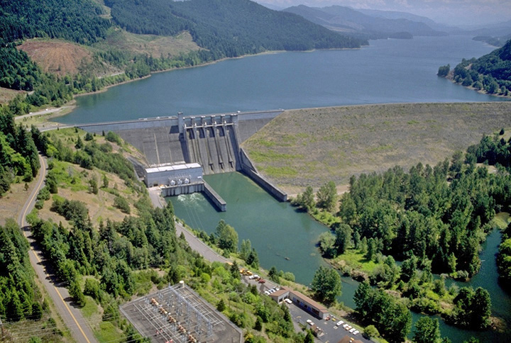
Figure 12.1: Lookout Point Dam on the Middle Fork Willamette River source: U.S. Army Corps of Engineers
Water resources systems tend to provide a variety of benefits, such as flood control, hydroelectric power, recreation, navigation, and irrigation. Each of these provides a benefit that can quantified, and there are also associated costs that can be quantified. A challenge engineers face is how to manage a system to balance the different uses. Mathematical optimization, which can take many forms, is employed to do this.
Introductions to linear programming and other forms of optimization are plentiful. For a background on the concepts and theories, refer to other references. An excellent, comprehensive reference is Water Resource Systems Planning and Management (Loucks & Van Beek, 2017), freely available online.
What follows is a demonstration of using some of these optimization methods, but no recap of the theory is provided. The examples here use linear systems, where the objective function and constraints are all linear functions of the decision variables.
The hydromisc package will need to be installed to access some of the data used below. If it is not installed, do so following the instructions on the github site for the package.
12.1 A simple linear system with two decision variables
12.1.1 Overview of problem formulation
One of the simplest systems to optimize is a linear system of two variables, which means a graphical solution in 2-d is possible. This first demonstration is one example, a reworking of a textbook example (Wurbs & James, 2002).
To set up a solution, three things must be described:
- the decision variables – the variables for which optimal values are sought
- the constraints – physical or other limitations on the decision variables (or combinations of them)
- the objective function – an expression, using the decision variables, of what is to be minimized or maximized.
12.1.2 Setting up an example
Example 12.1
To supply water to a community, there are two sources of water available with different levels of total dissolved solids (TDS): groundwater (TDS=980 mg/l) and surface water from a reservoir (TDS=100 mg/l). The first two constraints are that a total demand of water of 7,500 m\(^3\)must be met, and the delivered water (mixed groundwater and reservoir supplies) can have a maximum TDS of 500 mg/l. This is illustrated in Figure 12.2.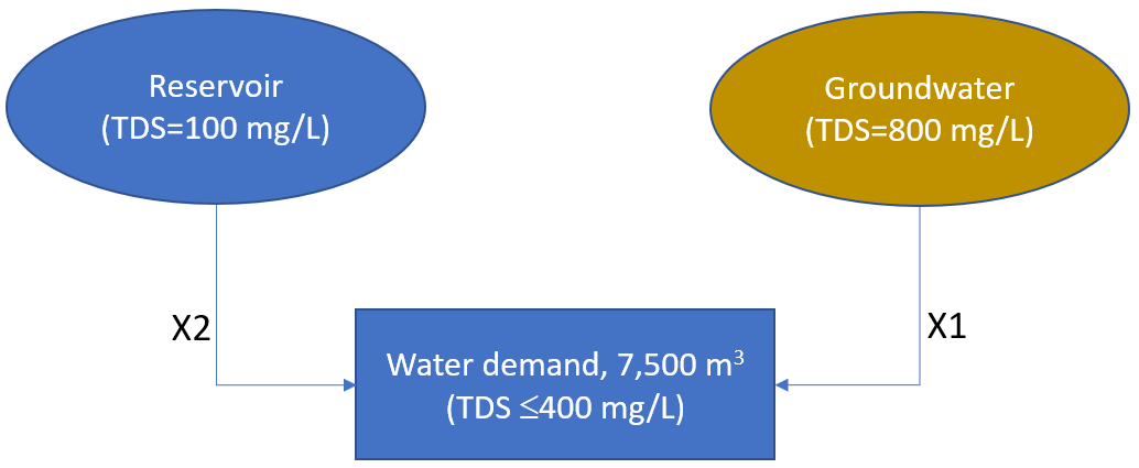
Figure 12.2: A schematic of the system for this example.
Two additional constraints are that groundwater withdrawal cannot exceed 4,000 m\(^3\) and reservoir withdrawals cannot exceed 7,500 m\(^3\). There are two decision variables: X1=groundwater and X2=reservoir supply. The objective is to minimize the reservoir withdrawal while meeting the constraints.
The TDS constraint is reorganized as: \[\frac{800~X1+100~X2}{X1+X2}\le 400~~~or~~~ 400~X1-300~X2\le 0\] Rewriting the other three constraints as functions of the decision variables: \[\begin{align*} X1+X2 \ge 7500 \\ X1 \le 4000 \\ X2 \le 7500 \end{align*}\]
Notice that the contraints are all expressed as linear functions of the decision variables (left side of the equations) and a value on the right.
12.1.3 Graphing the solution space
While this can only be done easily for systems with only two decision variables, a plot of the solution space can be done here by graphing all of the constrains and shading the region where all constraints are satisfied.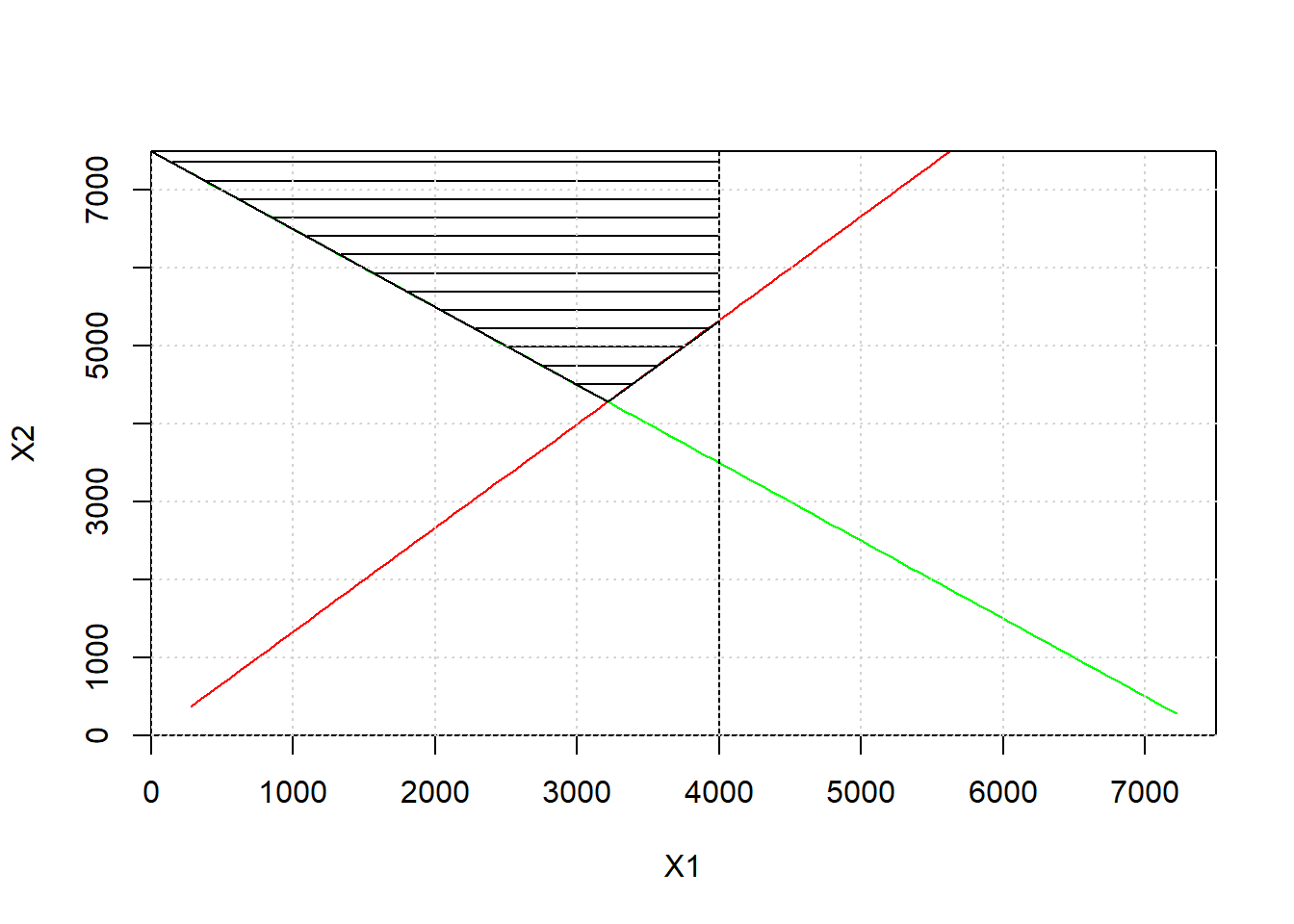
Figure 12.3: The solution space, shown as the cross-hatched area.
In the feasible region, it is clear that the minimum reservoir supply, X2, would be a little larger than 4,000 m\(^3\).
12.1.4 Setting up the problem in R
An R package useful for solving linear programming problems is the lpSolveAPI package. Install that if necessary, and also install the knitr and kableExtra packages, since thet are very useful for printing the many tables that linear programming involves.
Begin by creating an empty linear model. The (0,2) means zero constraints (they’ll be added later) and 2 decision variables. The next two lines just assign names to the decision variables. Because we will use many functions of the lpSolveAPI package, load the library first. Load the kableExtra package too.
library(lpSolveAPI)
library(kableExtra)
example.lp <- lpSolveAPI::make.lp(0,2)     # 0 constraints and 2 decision variables
ColNames <- c("X1","X2")
colnames(example.lp) <- ColNames           # Set the names of the decision variables
Now set up the objective function. Minimization is the default goal of this R function, but we’ll set it anyway to be clear. The second argument is the vector of coefficients for the decision variables, meaning X2 is minimized.
set.objfn(example.lp,c(0,1))
x <- lp.control(example.lp, sense="min") #save output to a dummy variable
The next step is to define the constraints. Four constraints were listed above. Additional constraints could be added that \(X1\ge 0\) and \(X2\ge 0\), however, variable ranges in this LP solver are [0,infinity] by default, so for this example and we do not need to include constraints for positive results. If necessary, decision variable valid ranges can be set using set.bounds().
Constraints are defined with the add.constraint command. Figure 12.4 provides an annotated example of the use of an add.constraint command.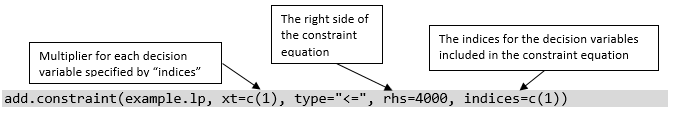
Figure 12.4: Annotated example of an add.constraint command.
Type ?add.constraint in the console for additional details.
The four constraints for this example are added with:
add.constraint(example.lp, xt=c(400,-300), type="<=", rhs=0, indices=c(1,2))
add.constraint(example.lp, xt=c(1,1), type=">=", rhs=7500)
add.constraint(example.lp, xt=c(1,0), type="<=", rhs=4000)
add.constraint(example.lp, xt=c(0,1), type="<=", rhs=7500)
That completes the setup of the linear model. You can view the model to verify the values you entered by typing the name of the model.
example.lp
#> Model name:
#>             X1    X2
#> Minimize     0     1
#> R1         400  -300  <=     0
#> R2           1     1  >=  7500
#> R3           1     0  <=  4000
#> R4           0     1  <=  7500
#> Kind       Std   Std
#> Type      Real  Real
#> Upper      Inf   Inf
#> Lower        0     0
If it has a large number of decision variables it only prints a summary, but in that case you can use write.lp(example.lp, "example_lp.txt", "lp") to create a viewable file with the model.
Now the model can be solved.
If the solver finds an optimal solution it will return a zero.
12.1.5 Interpreting the optimal results
View the final value of the objective function by retrieving it and printing it:
optimal_solution <- get.objective(example.lp)
print(paste0("Optimal Solution = ",round(optimal_solution,2),sep=""))
#> [1] "Optimal Solution = 4285.71"
For more detail, recover the values of each of the decision variables.
Next you can print the sensitivity report – a vector of M constraints followed by N decision variables. It helps to create a data frame for viewing and printing the results. Nicer printing is achieved using the kableExtra package. The signif function only keeps the specified number of significant figures, which makes for cleaner output.
sens <- get.sensitivity.obj(example.lp)$objfrom
results1 <- data.frame(variable=ColNames,value=signif(vars,5),gradient=as.integer(sens))
kbl(results1, booktabs = TRUE, caption = "Summary of output") |>
kable_styling(full_width = F)| variable | value | gradient |
|---|---|---|
| X1 | 3214.3 | -1 |
| X2 | 4285.7 | 0 |
The above shows decision variable values for the optimal solution. The Gradient is the change in the objective function for a unit increase in the decision variable. Here a negative gradient for decision variable \(X1\), the groundwater withdrawal, means that increasing the groundwater withdrawal will have a negative effect on the objective function, (to minimize \(X2\)): that is intuitive, since increasing groundwater withdrawal can reduce reservoir supply on a one-to-one basis.
To look at which constraints are binding, retrieve the $duals part of the output.
m <- length(get.constraints(example.lp)) #number of constraints
duals <- get.sensitivity.rhs(example.lp)$duals[1:m]
results2 <- data.frame(constraint=c(seq(1:m)),multiplier=signif(duals,5))
kbl(results2, booktabs = TRUE, digits = 5,
    caption = "Summary of constraints and multipliers", table.attr = "style='width:50%;'") |>
kable_styling(full_width = T, position = "center")| constraint | multiplier |
|---|---|
| 1 | -0.00143 |
| 2 | 0.57143 |
| 3 | 0.00000 |
| 4 | 0.00000 |
The multipliers for each constraint are referred to as Lagrange multipliers (or shadow prices). Non-zero values of the multiplier indicate a binding capability of that constraint, and the change in the objective function that would result from a unit change in that value. Zero values are non-binding, since a unit change in their value has no effect on the optimal result. For example, constraint 3, that \(X1 \le 4000\), with a multiplier of zero, could be changed (at least a small amount – there can be a limit after which it can become binding) with no effect on the optimal solution. Similarly, if constraint 2, \(X1+X2 \ge 7500\), were were increased, the objective function (the optimal reservoir supply) would also increase.
12.2 More complex linear programming: reservoir operation
Water resources systems are far too complicated to be summarized by two decision variables and only a few constraints, as above. Example 12.2 demonstrate how the same procedure can be applied to a slightly more complex system. This is a reformulation of an example from the same text as referenced above (Wurbs & James, 2002).
Example 12.2 A river flows into a storage reservoir where the operator must decide how much water to release each month. For simplicity, inflows will by described by a fixed sequence of 12 monthly flows. There are two downstream needs to satisfy: hydropower generation and irrigation diversions. Benefits are derived from these two uses: revenues are $ 800 per 10\(^6\)m\(^3\) of water diverted for irrigation, and $ 350 per 10\(^6\)m\(^3\) for hydropower generation. The objective is to determine the releases that will maximize the total revenue.
There are physical characteristics of the system that provide some constraints, and others are derived from basic physics, such as the conservation of mass. A schematic of the system is shown in Figure 12.5.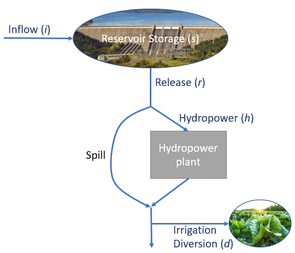
Figure 12.5: A schematic of the water resources system for this example.
| Month | Demand, 10\(^6\)m\(^3\) | Month | Demand, 10\(^6\)m\(^3\) | Month | Demand, 10\(^6\)m\(^3\) |
|---|---|---|---|---|---|
| Jan (1) | 0 | May (5) | 40 | Sep (9) | 180 |
| Feb (2) | 0 | Jun (6) | 130 | Oct (10) | 110 |
| Mar (3) | 0 | Jul (7) | 230 | Nov (11) | 0 |
| Apr (4) | 0 | Aug (8) | 250 | Dec (12) | 0 |
12.2.1 Problem summary
There are 48 decision variables in this problem, 12 monthly values for reservoir storage (s\(_1\)-s\(_{12}\)), release (r\(_1\)-r\(_{12}\)), hydropower generation (h\(_1\)-h\(_{12}\)), and agricultural diversion (d\(_1\)-d\(_{12}\)).
The objective function is to maximize the revenue, which is expressed by Equation (12.1). \[\begin{equation} Maximize~ x_0=\sum_{i=1}^{12}\left(350h_i+800d_i\right) \tag{12.1} \end{equation}\]
Constraints will need to be described to apply the limits to hydropower diversion and storage capacity, and to limit agricultural diversions to no more than the demand.
12.2.2 Setting up the problem in R
Create variables for the known or assumed initial values for the system.
penstock_cap <- 160        #penstock capacity in million m3/month
res_cap <- 550             #reservoir capacity in million m3
res_init_vol <- res_cap/2  #set initial reservoir capacity equal to half of capacity
irrig_dem <- c(0,0,0,0,40,130,230,250,180,110,0,0)
revenue_water <- 800       #revenue for delivered irrigation water, $/million m3
revenue_power <- 350       #revenue for power generated, $/million m3
A time series of 20 years (January 2000 through December 2019) of monthly flows for this exercise is included with the hydromisc package. Load that and extract the first 12 months to use in this example.
inflows_20years <- hydromisc::inflows_20years
inflows <- as.numeric(window(inflows_20years, start = c(2000, 1), end = c(2000, 12)))
It helps to illustrate how the irrigation demands and inflows vary, and therefore why storage might be useful in regulating flow to provide more reliable irrigation deliveries.
par(mgp=c(2,1,0))
ylbl <- expression(10 ^6 ~ m ^3/month)
plot(inflows, type="l", col="blue", xlab="Month", ylab=ylbl)
lines(irrig_dem, col="darkgreen", lty=2)
legend("topright",c("Inflows","Irrigation Demand"),lty = c(1,2), col=c("blue","darkgreen"))
grid()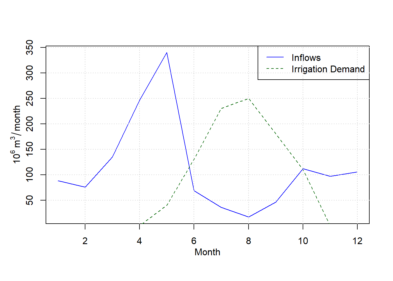
Figure 12.6: Inflows and irrigation demand.
12.2.3 Building the linear model
Following the same steps as for a simple 2-variable problem, begin by setting up a linear model. Because there are so many decision variables, it helps to add names to them.
reser.lp <- make.lp(0,48)
DecisionVarNames <- c(paste0("s",1:12),paste0("r",1:12),paste0("h",1:12),paste0("d",1:12))
colnames(reser.lp) <- DecisionVarNames| Decision Variables | Indices (columns) |
|---|---|
| Storage (s1-s12) | 1-12 |
| Release (r1-r12) | 13-24 |
| Hydropower (h1-h12) | 25-36 |
| Irrigation diversion (d1-d12) | 37-48 |
Using these indices as a guide, set up the objective function and initialize the linear model. While not necessary, redirecting the output of the lp.control to a variable prevents a lot of output to the console. The following takes the revenue from hydropower and irrigation (in $ per 10\(^6\)m\(^3\)/month), multiplies them by the 12 monthly values for the hydropower flows and the irrigation deliveries, and sets the objective to maximize their sum, as described by Equation (12.1).
set.objfn(reser.lp,c(rep(revenue_power,12),rep(revenue_water,12)),indices = c(25:48))
x <- lp.control(reser.lp, sense="max")
With the LP setup, the constraints need to be applied. Negative releases, storage, or river flows don’t make sense, so they all need to be positive, so \(s_t\ge0\), \(r_t\ge0\), \(h_t\ge0\) for all 12 months, but because the lpSolveAPI package assumes all decision variables have a range of \(0\le x\le \infty\) these do not need to be explicitly added as constraints. When using other software packages these may need to be included.
12.2.3.1 Constraints 1-12: Maximum storage
The maximum capacity of the reservoir cannot be exceeded in any month, or \(s_t\le 550\) for all 12 months. This can be added in a simple loop:
12.2.3.2 Constraints 13-24: Irrigation diversions
The irrigation diversions should never exceed the demand. While for some months they are set to zero, since decision variables are all assumed non-negative, we can just assign all irrigation deliveries using the \(\le\) operator.
12.2.3.3 Constraints 25-36: Hydropower capacity
Hydropower release cannot exceed the penstock capacity in any month: \(h_t\le 160\) for all 12 months. This can be done following the example above for the maximum storage constraint
12.2.3.4 Constraints 37-48: Reservoir release
Reservoir release must equal or exceed irrigation deliveries, which is another way of saying that the water remaining in the river after the diversion cannot be negative. In other words \(r_1-d_1\ge 0\), \(r_2-d_2\ge 0\), … for all 12 months. For constraints involving more than one decision variable the constraint equations look a little different, and keeping track of the indices associated with each decision variable is essential.
12.2.3.5 Constraints 49-60: Hydropower generation
Hydropower generation will be less than or equal to reservoir release in every month, or \(r_1-h_1\ge 0\), \(r_2-h_2\ge 0\), … for all 12 months.
12.2.3.6 Constraints 61-72: Conservation of mass
Finally, considering the reservoir, the inflow minus the outflow in any month must equal the change in storage over that month. That can be expressed in an equation with decision variables on the left side as: \[s_t-s_{t-1}+r_t=inflow_t\] where \(t\) is a month from 1-12 and \(s_t\) is the storage at the end of month \(t\). We need to use the initial reservoir volume, \(s_0\) (given above in the problem statement) for the first month’s mass balance, so the above would become \(s_1-s_0+r_1=inflow_1\), or \(s_1+r_1=inflow_1+s_0\). All subsequent months can be assigned in a loop,
add.constraint(reser.lp, xt=c(1,1), type="=", rhs=inflows[1]+res_init_vol, indices=c(1,13))
for (i in seq(2,12)) {
  add.constraint(reser.lp, xt=c(1,-1,1), type="=", rhs=inflows[i], indices=c(i,i-1,i+12))
}write.lp(reser.lp, "reservoir_LP.txt", "lp") to create a file (readable using any text file viewer, like Notepad++) with all of the model details. It can also be read into R with the read.lp command to load the complete LP. The beginning of the file for this LP looks like:
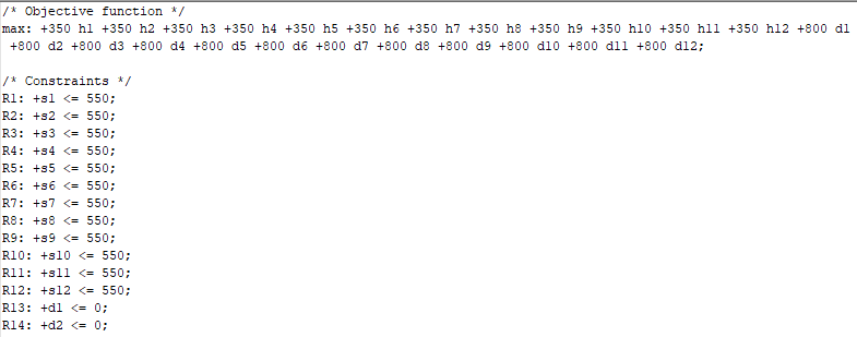
Figure 12.7: The top of the linear model file produced by write.lp().
12.2.3.7 Solving the model and interpreting output
Solve the LP and retrieve the value of the objective function.
To look at the hydropower generation, and to see how often spill occurs, it helps to view the associated decision variables (as noted above, these are indices 12-24 and 25-36).
vars <- get.variables(reser.lp)       # retrieve decision variable values
results0 <- data.frame(variable=DecisionVarNames,value=vars)
r0 <- cbind(month.abb, results0[13:24, ], results0[25:36, ])
rownames(r0) <- c()
column_names <- c("Month", "Reservoir Release", paste0("10$^6$m$^3$"),
                  "Hydropower Diversion", paste0("10$^6$m$^3$"))
kbl(r0, booktabs = TRUE, digits = 1, col.names=column_names,
    caption = "Monthly reservoir releases and amount used for hydropower") |>
kable_styling(bootstrap_options = c("striped","condensed"),full_width = F)| Month | Reservoir Release | 10\(^6\)m\(^3\) | Hydropower Diversion | 10\(^6\)m\(^3\) |
|---|---|---|---|---|
| Jan | r1 | 160.0 | h1 | 160.0 |
| Feb | r2 | 160.0 | h2 | 160.0 |
| Mar | r3 | 160.0 | h3 | 160.0 |
| Apr | r4 | 89.4 | h4 | 89.4 |
| May | r5 | 40.0 | h5 | 40.0 |
| Jun | r6 | 130.0 | h6 | 130.0 |
| Jul | r7 | 230.0 | h7 | 160.0 |
| Aug | r8 | 197.6 | h8 | 160.0 |
| Sep | r9 | 160.0 | h9 | 160.0 |
| Oct | r10 | 112.0 | h10 | 112.0 |
| Nov | r11 | 97.0 | h11 | 97.0 |
| Dec | r12 | 105.5 | h12 | 105.5 |
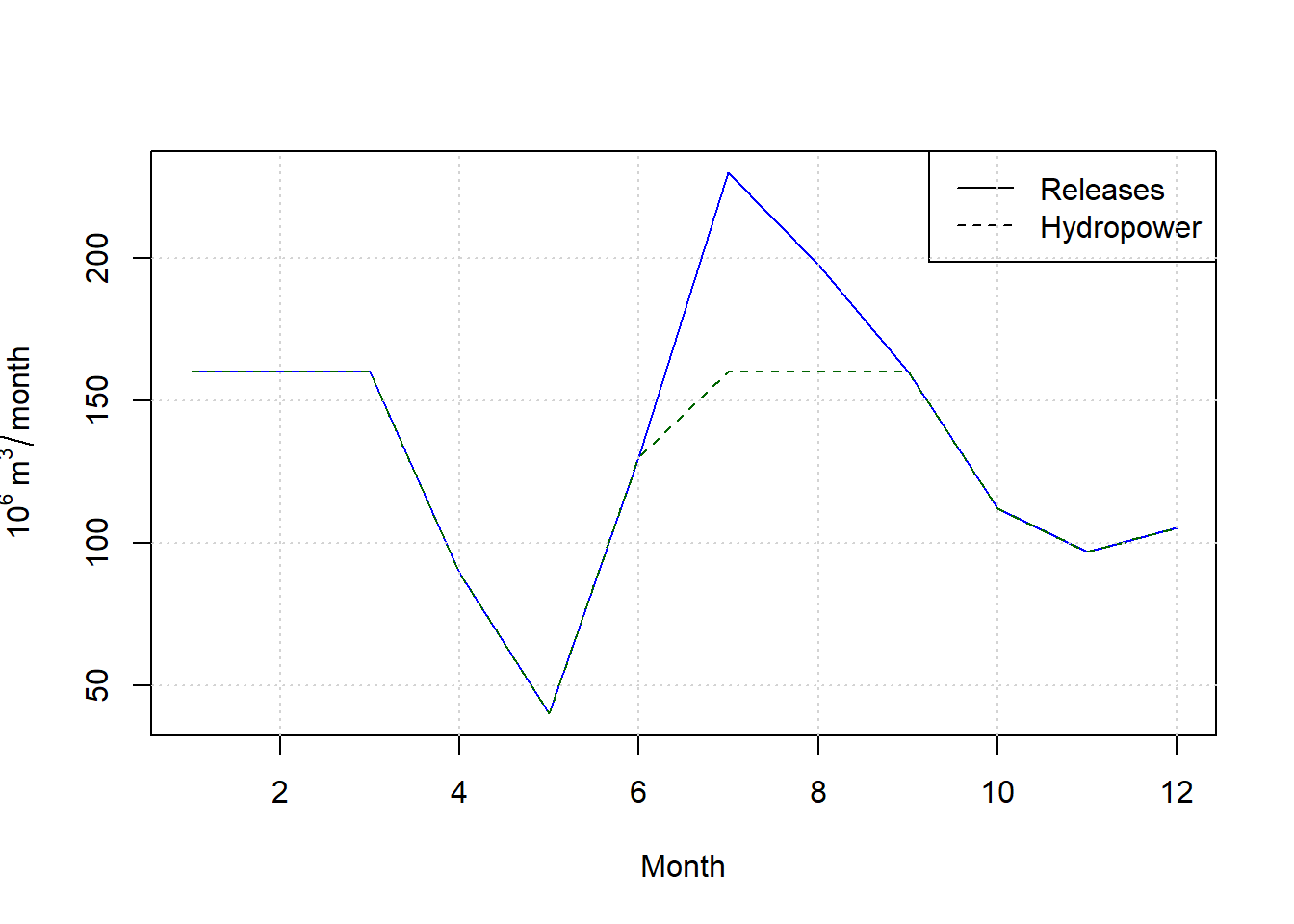
Figure 12.8: Reservoir releases and hydropower water use for optimal solution.
For this optimal solution, the releases exceed the capacity of the penstock supplying the hydropower plant in July and August, meaning there would be reservoir spill during those months.
Another part of the output that is important is to what degree irrigation demand is met. the irrigation delivery is associated with decision variables with indices 37-48.| Month | Decision variable | Delivery, 10\(^6\)m\(^3\) | Demand, 10\(^6\)m\(^3\) |
|---|---|---|---|
| Jan | d1 | 0 | 0 |
| Feb | d2 | 0 | 0 |
| Mar | d3 | 0 | 0 |
| Apr | d4 | 0 | 0 |
| May | d5 | 40 | 40 |
| Jun | d6 | 130 | 130 |
| Jul | d7 | 230 | 230 |
| Aug | d8 | 198 | 250 |
| Sep | d9 | 160 | 180 |
| Oct | d10 | 110 | 110 |
| Nov | d11 | 0 | 0 |
| Dec | d12 | 0 | 0 |
August and September see a shortfall in irrigation deliveries where full demand is not met.
Finally, finding which constraints are binding can provide insights into how a system might be modified to improve the optimal solution. This is done similarly to the simpler problem above, by retrieving the duals portion of the sensitivity results. To address the question of whether the size of the reservoir is a binding constraint, that is, whether increasing reservoir size would improve the optimal results, only the first 12 constraints are printed.
m <- length(get.constraints(reser.lp))             # retrieve the number of constraints
duals <- get.sensitivity.rhs(reser.lp)$duals[1:m]
results2 <- data.frame(Constraint=c(seq(1:m)),Multiplier=duals)
kbl(results2[1:12,], booktabs = TRUE, caption = "Multipliers for the constraint of reservoir capacity", table.attr = "style='width:50%;'") |>
kable_styling(bootstrap_options = c("striped","condensed"),full_width = T, position = "center")| Constraint | Multiplier |
|---|---|
| 1 | 0 |
| 2 | 0 |
| 3 | 0 |
| 4 | 0 |
| 5 | 450 |
| 6 | 0 |
| 7 | 0 |
| 8 | 0 |
| 9 | 0 |
| 10 | 0 |
| 11 | 0 |
| 12 | 0 |
For this example, in only one month would a larger reservoir have a positive impact on the maximum revenue.
12.3 More Realistic Reservoir Operation: non-linear programming
While the simple examples above illustrate how an optimal solution can be determined for a linear (and deterministic) reservoir system, in reality reservoirs are much more complex. Most reservoir operation studies use sophisticated software to develop and apply Rule Curves for reservoirs, aiming to optimally store and release water, preserving the storage pools as needed. Figure 12.9 shows how reservoir volumes are managed.
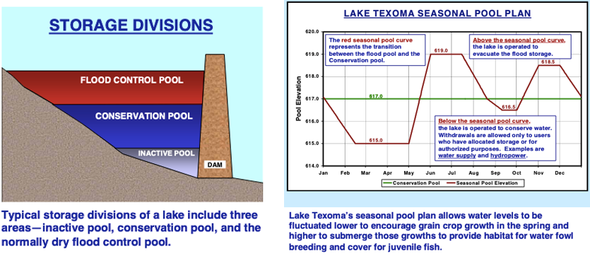
Figure 12.9: Sample reservoir operating goals U.S. Army Corps of Engineers
Many rule curves depend on the condition of the system at some prior time. Figure 12.10 shows a rule curve used to operate Folsom Reservoir on the American River in California, where the target storage depends on the total upstream storage available.
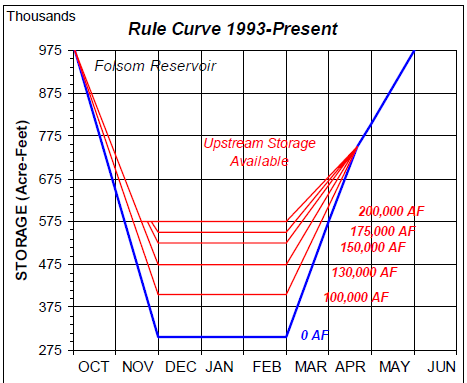
Figure 12.10: Multiple rule corves based on upstream storage U.S. Army Corps of Engineers Report RD-48
One method for deriving an optimal solution for the nonlinear and random processes in a water resources system is stochastic dynamic programming (SDP). Like LP, SDP uses algorithms that optimize an objective function under specified constraints. However, SDP can accommodate non-linear, dynamic outcomes, such as those associated with floods risks or other stochastic events. SDP can combine the stochastic information with reservoir management actions, where the outcome of decisions can be dependent on the state of the system (as in Figure 12.10). Constraints can be set to be met a certain percentage of the time, rather than always.
12.3.1 Reservoir operation
While SDP is a topic that is far more advanced than what will be covered here, one R package will be introduced. For reservoir optimization, the R package reservoir can use SDP to derive an optimal operating rule for a reservoir given a sequence of inflows using a single or multiple constraints. The package can also take any derived rule curve and operate a reservoir using it, which is what will be demonstrated here.
First, place the optimal releases, according to the LP above, into a new vector to be used as a set of target releases for the reservoir operation.
The reservoir can be operated (for the same 12-month period, with the same 12 inflows as above) with a single command.
The total revenue from hydropower generation and irrigation deliveries is computed as follows.
irrig_releases <- pmin(x$releases,irrig_dem)
irrig_benefits <- sum(irrig_releases*revenue_water)
hydro_releases <- pmin(x$releases,penstock_cap)
hydro_benefits <- hydro_releases*revenue_power
sum(irrig_benefits,hydro_benefits)
#> [1] 1230930
Unsurprisingly, this produces the same result as with the LP example.
12.3.2 Performing stochastic dynamic programming
The optimal releases, or target releases, were established based on a single year. the SDP in the reservoir package can be used to determine optimal releases based on a time series of inflows. Here the entire 20-year inflow sequence is used to generate a multiobjective optimal solution for the system. A weighting must be applied to describe the importance of meeting different parts of the objective function. The target release(s) cannot be zero, so a small constant is added.
weight_water <- revenue_water/(revenue_water + revenue_power)
weight_power <- revenue_power/(revenue_water + revenue_power)
z <- reservoir::sdp_multi(inflows_20years, cap=res_cap, target = irrig_dem+0.01,
                          R_max = penstock_cap, spill_targ = 0.95,
                          weights = c(weight_water, weight_power, 0.00),
                          loss_exp = c(1, 1, 1), tol=0.99, S_initial=0.5, plot=FALSE)
irrig_releases2 <- pmin(z$releases,irrig_dem)
irrig_benefits2 <- sum(irrig_releases2*revenue_water)
hydro_releases2 <- pmin(z$releases,penstock_cap)
hydro_benefits2 <- hydro_releases2*revenue_power
sum(irrig_benefits2,hydro_benefits2)/20
#> [1] 911240For a 20-year period, the average annual revenue will always be less than that for a single year where the optimal releases are designed based on that same year.