Chapter 6 Momentum in water flow

When moving water changes direction or velocity, an external force must be associated with the change. In civil engineering infrastructure this is ubiquitous and the forces associated with this must be accounted for in design.

Figure 6.1: Water pipe on Capitol Hill, Seattle.

6.1 Equations of linear momentum

Newton’s law relates the forces applied to a body to the rate of change of linear momentum, as in Equation (6.1) \[\begin{equation} \sum{\overrightarrow{F}}=\frac{d\left(m\overrightarrow{V}\right)}{dt} \tag{6.1} \end{equation}\]

For fluid flow in a hydraulic system carrying a flow Q, the equation can be written in any linear direction (x-direction in this example) as in Equation (6.2).

\[\begin{equation} \sum{F_x}=\rho{Q}\left(V_{2x}-V_{1x}\right) \tag{6.2} \end{equation}\] where \(\rho{Q}\) is the mass flux through the system, \(V_{1x}\) is the velocity in the x-direction where flow enters the system, and \(V_{2x}\) is the velocity in the x-direction where flow leaves the system. \(\sum{F_x}\) is the vector sum of all external forces acting on the system in the x-direction.

It should be noted that the values of V are the average cross-sectional velocity. A momentum correction factor (\(\beta\)), can be applied when the velocity is highly non-uniform across the cross-section. In nearly all civil engineering applications the adjustment factor is close enough to 1 where it is ignored in the calculations.

6.2 The momentum equation in pipe design

One of the most common civil engineering applications of the momentum equation is providing the lateral restraint where a pipe bend occurs. One approach to provide the external force to keep the pipe in equilibrium is to use a thrust block, as illustrated in Figure 6.2 (Ductile Iron Pipe Research Association, 2016).

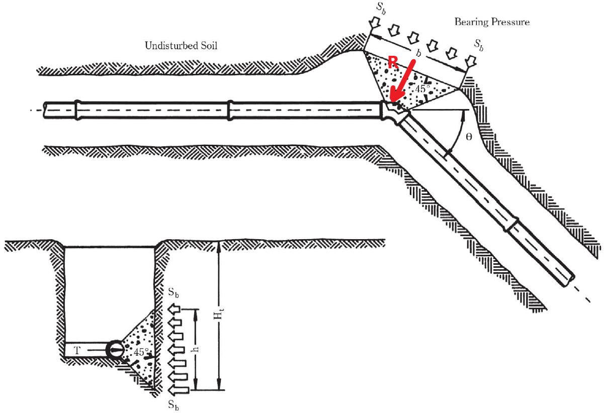
Figure 6.2: A sketch of a pipe bend with a thrust block.

Example 6.1 A horizontal 18-inch diameter pipe carries flow Q of water at 68\(^\circ\)F with a pressure of 60 psi and encounters a bend of angle \(\theta=30^\circ\). Show how the reaction force, R varies with the flow rate through the bend for flows up to 20 ft³/s. Ignore head loss through the bend.

Taking the control volume to be the bend, the external forces acting on the bend are shown in Figure 6.3.

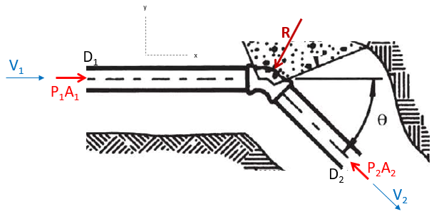
Figure 6.3: External forces on the pipe.

Note that if the pipe were not horizontal, the weight of the water in the pipe would also need to be included.

Including all of the external forces in the x-direction on left side of Equation (6.2) and recognizing that V_1x=V₁ and V_2x=V₂cos\(\theta\) produces: \[P_1A_1-P_2A_2cos\theta-R_x=\rho{Q}\left(V_{2}cos\theta-V_{1}\right)\] Rearranging to solve for R_x gives Equation (6.3). \[\begin{equation} R_x=P_1A_1-P_2A_2cos\theta-\rho{Q}\left(V_{2}cos\theta-V_{1}\right) \tag{6.3} \end{equation}\] Similarly in the y-direction Equation (6.4) can be assembled, noting that V_1y=0 and V_2y=\(-\)V₂sin\(\theta\) . \[\begin{equation} R_y=P_2A_2sin\theta-\rho{Q}\left(-V_{2}sin\theta\right) \tag{6.4} \end{equation}\]

This can be set up in R in many ways, such as the following.

#Input Data -- ensure units are consistent in ft, lbf (pound force), sec
D1 <- units::set_units(18/12, ft)
D2 <- units::set_units(18/12, ft)
P1 <- units::set_units(60*144, lbf/ft^2) #convert psi to lbf/ft^2
P2 <- units::set_units(60*144, lbf/ft^2)
theta <- 30*(pi/180) #convert to radians for sin, cos functions
rho <- hydraulics::dens(T=68, units="Eng", ret_units = TRUE)

# calculations - vary flow from 0 to 20 ft^3/s
Q <- units::set_units(seq(0,20,1), ft^3/s)
A1 <- pi/4*D1^2
A2 <- pi/4*D2^2
V1 <- Q/A1
V2 <- Q/A2
Rx <- P1*A1-P2*A2*cos(theta)-rho*Q*(V2*cos(theta)-V1)
Ry <- P2*A2*sin(theta)-rho*Q*(-V2*sin(theta))
R <- sqrt(Rx^2 + Ry^2)
plot(Q,R)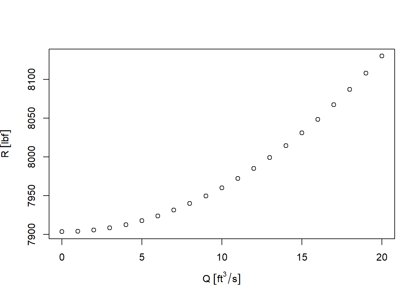

When Q=0, only the pressure terms contribute to R. This plot shows that for typical water main conditions the change in direction of the velocity vectors adds a small amount (less than 3% in this example) to the calculated R value. This is why design guidelines for water mains often neglect the velocity term in Equation (6.2). In other industrial or laboratory conditions it may not be valid to neglect that term.