Chapter 9 Fate of precipitation

As precipitation falls and can be caught on vegetation (interception), percolate into the ground (infiltration), return to the atmosphere (evaporation), or become available as runoff (if accumulating as rain or snow). The landscape (land cover and topography) and the time scale of study determine what processes are important. For example, for estimating runoff from an individual storm, interception is likely to be small, as is evaporation. On an annual average over large areas, evaporation will often be the largest component.

Comprehensive hydrology models will estimate abstractions due to infiltration and interception, either by simulating the physics of the phenomenon or by using a lumped parameter that accounts for the effects of abstractions on runoff.

The hydromisc package will need to be installed to access some of the code and data used below. If it is not installed, do so following the instructions on the github site for the package.

9.1 Interception

Figure 9.1: Rain interception by John Robert McPherson, CC BY-SA 4, via Wikimedia Commons

Interception of rainfall is generally small during individual storms (0.5-2 mm), so it is often ignored, or lumped in with other abstractions, for analyses of flood hydrology. For areas characterized by low intensity rainfall and heavy vegetation, interception can account for a larger portion of the rainfall (for example, up to 25% of annual rainfall in the Pacific Northwest) (McCuen, 2016).

9.2 Infiltration

The movement of water through a saturated soil column is governed by Darcy’s law. (9.1). \[\begin{equation} q~=~ -K\frac{\partial H}{\partial s} \tag{9.1} \end{equation}\] where q is the flow of water per unit area (L/T), K is the hydraulic conductivity (L/T), H is the hydraulic head (L) and s is the distance along a flow path. Because infiltration into soils often begins with unsaturated conditions, K becomes a function of water content and hydraulic head. The solution becomes complicated, and empirical formulations are used.

9.2.1 Horton infiltration equation

An early empirical equation describing infiltration rate into soils was developed by Horton (Horton, R.E., 1939), which takes the form of Equation (9.2). \[\begin{equation} f_p~=~ f_c + \left(f_0 - f_c\right)e^{-kt} \tag{9.2} \end{equation}\] This describes a potential infiltration rate, \(f_p\), beginning at a maximum \(f_0\) and decreasing with time toward a minimum value \(f_c\) at a rate described by the decay constant \(k\). \(f_c\) is also equal to the saturated hydraulic conductivity, \(K_s\), of the soil. If rainfall rate exceeds \(f_c\) then this equation describes the actual infiltration rate with time. If periods of time have rainfall less intense than \(f_c\) it is convenient to integrate this to relate the total cumulative depth of water infiltrated, \(F\), and the actual infiltration rate, \(f_p\), as in Equation (9.3). \[\begin{equation} F~=~\left[\frac{f_c}{k}ln\left(f_0-f_c\right)+\frac{f_0}{k}\right]-\frac{f_c}{k}ln\left(f_p-f_c\right)-\frac{f_p}{k} \tag{9.3} \end{equation}\]

Parameters for the Horton, Green-Ampt, and other infiltration models can be derived from observed infiltration data using the R package HydroMe. Fitting the Horton equation to observed data is demonstrated here using a small sample from the infilt data set included with the HydroMe package which is saved in a spreadsheet wrapped into the hydromisc package. While HydroMe includes a function to return parameters, this can also be done manually as shown here.

Example 9.1 Fit a Horton infiltration model to measured infiltration data, then use the derived parameters to plot the infiltration rate over time.

First, read in the data sample.

# path to sample spreadsheet
datafile <- system.file("extdata", "infilt_field_data.xlsx", package="hydromisc")
infilt_data <- readxl::read_excel(datafile)

Set up a function for the Horton equation and use the built in stats package function nls to solve for the parameters. This works with column names of ‘Time’ and ‘Rate’.

horton <- function(time, fc, f0, k) {
  fc + (f0 - fc) * exp(-k * time)
}
horton_fit <- stats::nls(Rate ~ horton(Time, fc, f0, k), data = infilt_data, 
                  start = list(fc=0.2, f0=1, k=0.1))
coef(horton_fit)
#>         fc         f0          k 
#> 0.52816668 1.25076319 0.05102829

Plot the results of the fit with the observations.

infilt_data$Rate_Horton <- predict(horton_fit, list(x = infilt_data$Time))
plot(infilt_data$Time,infilt_data$Rate, pch=1, 
     xlab = "Time, min", ylab = "Infiltration rate, cm/hr")
lines(infilt_data$Time, infilt_data$Rate_Horton, lty = 1)
legend("topright", legend = c("Obs.","Horton"), pch = c(1, NA), lty = c(NA, 1))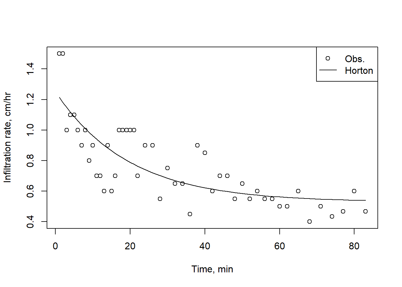

Figure 9.2: A Horton infiltration curve fit to experimental observations.

9.2.2 Green-Ampt infiltration model

A more physically based relationship to describe infiltration rate is the Green-Ampt model (Green & Ampt, 1911). It is based on the physical laws describing the propogation of a wetting front downward through a soil column under a ponded water surface. The Green-Ampt relationship is expressed either in terms of infiltration rate, \(f_p\) or cumulative infiltration, F, as in Equations (9.4) and (9.5). \[\begin{equation} f_p~=~K_s\left[1~+~\frac{\Delta\theta~\Psi_f}{F}\right] \tag{9.4} \end{equation}\] \(\Delta\theta=\left(n-\theta_i\right)\) where n is effective porosity and \(\theta\) is the initial water content. \(\Psi\) is the capillary potential or wetting front suction head. \[\begin{equation} K_st~=~F-\left(n-\theta_i\right)\Psi_f~ln\left[1+\frac{F}{\left(n-\theta_i\right)\Psi_f}\right] ~=~ F-N_s~ln\left[1+\frac{F}{N_s}\right] \tag{9.5} \end{equation}\] The parameter \(N_s=\left(n-\theta_i\right)\Psi_f\) is referred to as the matric potential. Different references use different symbols for these terms. These equations assume ponding begins at t=0, meaning rainfall rate exceeds \(K_s\). When rainfall rates are less than that, adjustments to the method are used. Typical parameter values are shown in the table below.

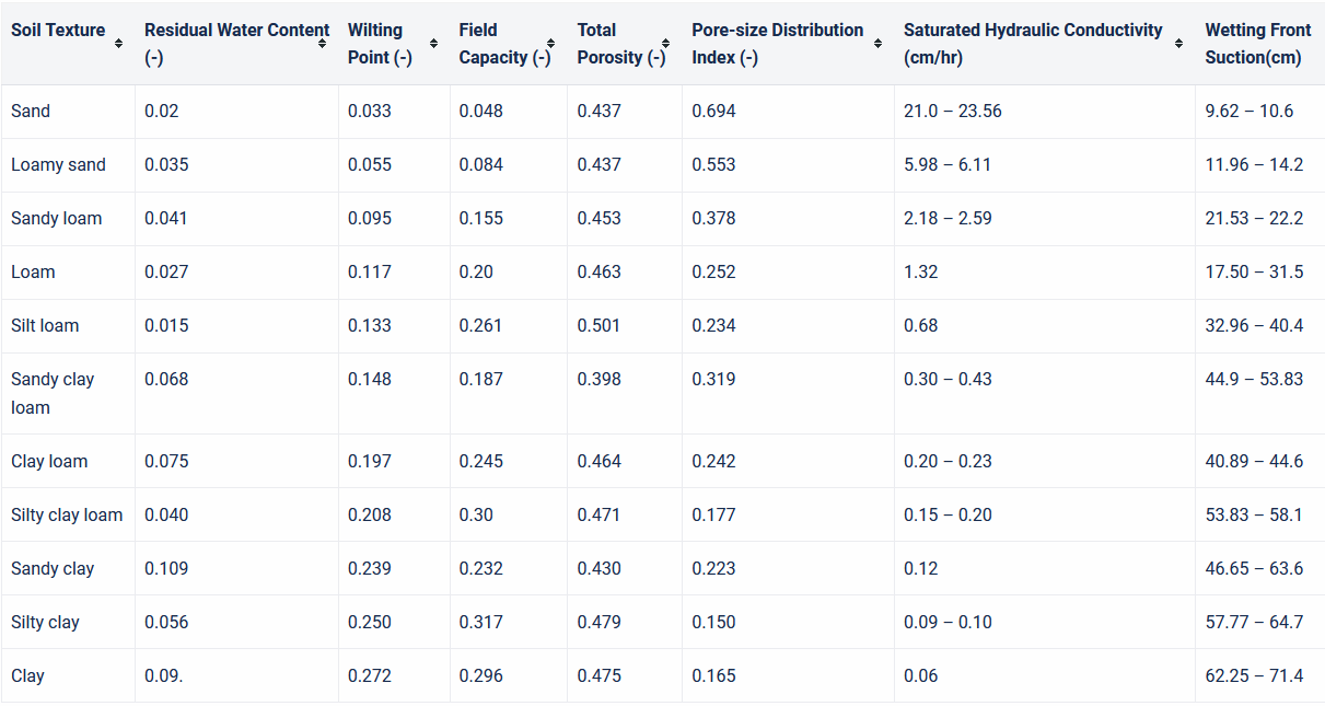
Figure 9.3: Green-Ampt Parameter Estimates and Ranges based on Soil Texture USACE

Example 9.2 Fit a Green-Ampt infiltration model to measured infiltration data, then use the derived parameters to plot the infiltration rate over time.

For convenience, this uses the same infiltration data as in the prior example. Because the Green-Ampt formulation needs cumulative infiltration depth, F, first create a column of this in the data frame.

# Add a column for incremental time
infilt_data <- infilt_data |> dplyr::mutate(dt = Time - dplyr::lag(Time))
# Add value to first row
infilt_data$dt[1] <- infilt_data$Time[1]
# Add a column for cumulative infiltration
infilt_data$Cumul_Infilt <- cumsum(infilt_data$Rate * infilt_data$dt)

Because the Green-Ampt model comprises implicit, nonlinear equations they cannot be solved directly, as could be done with the Horton equation. Combining the base uniroot function for solving an implicit equation with the non-linear fitting capabilities of the Flexible Modelling Environment FME package makes this possible in R.

First, define a function that finds cumulative infiltration, Fp, for a given time and the Green-Ampt parameters K and Ns in (9.5) (rearranged to solve for zero).

GA_infilt <- function(time, parms) {
    with(as.list(parms), {
      # function to solve for zero
      uniroot(function(Fp) Fp - K*time - Ns * log(1 + Fp/Ns), 
              interval = c(0, 1e3),
              tol = 1.e-6)$root
    })
  }

Now set up the function to optimize the parameters for all times, with the goal to minimize the square root of the squared differences. Any other function could be used to minimize the difference by changing the last line of the function. Then use the FME modFit function to find the optimal parameters.

GA_min <- function(ps) {
  K <- ps[1]
  Ns <- ps[2]
  GA_fit <- sapply(infilt_data$Time, GA_infilt, parms = c(K = K, Ns = Ns))
  sqrt((GA_fit - infilt_data$Cumul_Infilt)^2)
}

#Set initial parameter values and run minimization function for the best parameter set
parms_start <- c(1, 0.5)
GA_out <- FME::modFit(f = GA_min, p = parms_start, lower = c(0, 0), 
                  upper = c(Inf, Inf))
fitted_parms <- setNames(GA_out$par, c("K","Ns"))
fitted_parms
#>         K        Ns 
#> 0.5656739 4.8610322

Finally, use the best fit parameters to generate a sequence of cumulative infiltration values using (9.5) and infiltration rate using (9.4), plotting the results along with the constant rate (average) infiltration for the observation period.

fitted_F <- sapply(infilt_data$Time, GA_infilt, parms = fitted_parms)
infilt_data$Rate_GA <- fitted_parms[['K']] * (1 + fitted_parms[['Ns']]/fitted_F)

# Make a plot
plot(infilt_data$Time,infilt_data$Rate, pch=1, xlab = "Time, min", ylab = "Infiltration rate, cm/hr")
lines(infilt_data$Time, infilt_data$Rate_GA, lty = 2)
abline(h = tail(infilt_data$Cumul_Infilt, 1)/tail(infilt_data$Time, 1))
legend("topright", legend = c("Obs.","Green-Ampt","Constant"), pch = c(1, NA, NA), lty = c(NA, 2, 1))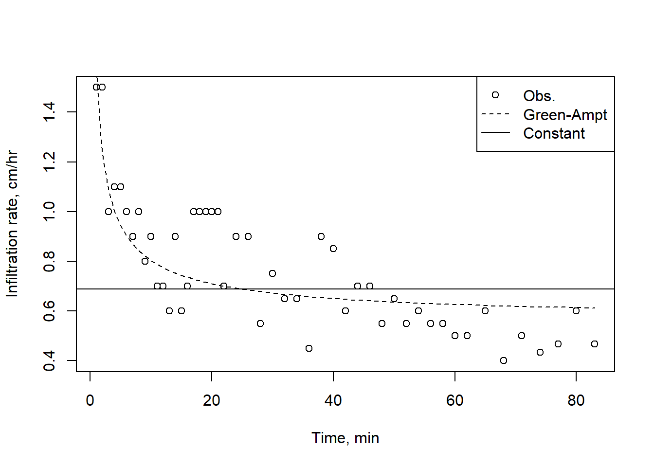

Figure 9.4: A Green-Ampt curve fit, with the average constant rate.

9.2.3 The NRCS method

The most widely used method for estimating infiltration is the NRCS method, described in detail in the NRCS document Estimating Runoff Volume and Peak Discharge.This method describes the direct runoff (as a depth), \(Q\), resulting from a precipitation event, \(P\), as in Equation (9.6). \[\begin{equation} Q~=~\frac{\left(P-I_a\right)^2}{\left(P-I_a\right)+S} \tag{9.6} \end{equation}\] \(S\) is the maximum retention of water by the soil column and \(I_a\) is the initial abstraction, commonly estimated as \(I_a=0.2S\). Substituting this into Equation (9.6) produces Equation (9.7). \[\begin{equation} Q~=~\frac{\left(P-0.2~S\right)^2}{\left(P+0.8~S\right)} \tag{9.7} \end{equation}\] This relationship applies as long as \(P>0.2~S\); Q=0 otherwise. Values for S are derived from a Curve Number (CN), which summarizes the land cover, soil type and condition: \[CN=\frac{1000}{10+S}\] where \(S\), and subsequently \(Q\), are in inches. Equation (9.7) can be rearranged to a form similar to those for the Horton and Green-Ampt equations for cumulative infiltration, \(F\). \[F~=~\frac{\left(P-0.2~S\right)S}{P+0.8~S}\].

9.3 Evaporation

Evaporation is simply the change of water from liquid to vapor state. Because it is difficult to separate evaporation from the soil from transpiration from vegetation, it is usually combined into Evapotranspiration, or ET; see Figure 9.5.

Figure 9.5: Schematic of ET, from CIMIS

ET can be estimated in a variety of ways, but it is important first to define three types of ET: - Potential ET, \(ET_p\) or \(PET\): essentially the same as the rate that water would evaporate from a free water surface. - Reference crop ET, \(ET_{ref}\) or \(ET_0\): the rate water evaporates from a well-watered reference crop, usually grass of a standard height. - Actual ET, \(ET\): this is the water used by a crop or other vegetation, usually calculated by adjusting the \(ET_0\) term by a crop coefficient that accounts for factors such as the plant height, growth stage, and soil exposure.

Estimating \(ET_0\) can be as uncomplicated as using the Thornthwaite equation, which depends only on mean monthly temperatures, to the Penman-Monteith equation, which includes solar and longwave radiation, wind and humidity effects, and reference crop (grass) characteristics. Inclusion of more complexity, especially where observations can supply the needed input, produces more reliable estimates of \(ET_0\).One of the most common implementations of the Penman-Monteith equation is the version of the FAO (FAO Irrigation and drainage paper 56, or FAO56) (Allen & United Nations, 1998). Refer to FAO56 for step-by-step instructions on determining each term in the Penman-Monteith equation, Equation (9.8). \[\begin{equation} \lambda~ET~=~\frac{\Delta\left(R_n-G\right)+\rho_ac_p\frac{\left(e_s-e_a\right)}{r_a}}{\Delta+\gamma\left(1+\frac{r_s}{r_a}\right)} \tag{9.8} \end{equation}\]

Open water evaporation can be calculated using the original Penman equation (1948): \[\lambda~E_p~=~\frac{\Delta~R_n+\gamma~E_a}{\Delta~+~\gamma}\] where \(R_n\) is the net radiation available to evaporate water and \(E_a\) is a mass transfer function usually including humidity (or vapor pressure deficit) and wind speed. \(\lambda\) is the latent heat of vaporization of water. A common implementation of the Penman equation is \[\begin{equation} \lambda~E_p~=~\frac{\Delta~R_n+\gamma~6.43\left(1+0.536~U_2\right)\left(e_s-e\right)}{\Delta~+~\gamma} \tag{9.9} \end{equation}\] Here \(E_p\) is in mm/d, \(\Delta\) and \(\gamma\) are in \(kPa~K^{-1}\), \(R_n\) is in \(MJ~m^{−2}~d^{−1}\), \(U_2\) is in m/s, and \(e_s\) and \(e\) are in kPa. Variables are as defined in FAO56.

Open water evaporation can also be calculated using a modified version of the Penman-Monteith equation (9.8). In this latter case, vegetation coefficients are not needed, so Equation (9.8) can be used with \(r_s=0\) and \(r_a=251/(1+0.536~u_2)\), following Thom & Oliver, 1977.

The R package Evaporation has functions to calculate \(ET_0\) using this and many other functions. This is especially useful when calculating PET over many points or through a long time series.

9.4 Snow

9.4.1 Observations

In mountainous areas a substantial portion of the precipitation may fall as snow, where it can be stored for months before melting and becoming runoff. Any hydrologic analysis in an area affected by snow must account for the dynamics of this natural reservoir and how it affects water supply. In the Western U.S., the most comprehensive observations of snow are part of the SNOTEL (SNOw TELemetry) network.

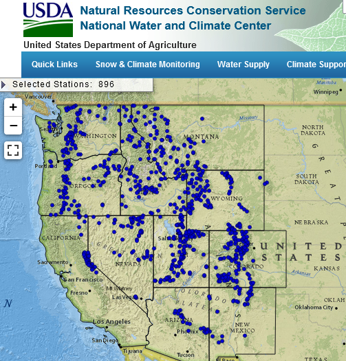
Figure 9.6: The SNOTEL network.

9.4.2 Basic snowmelt theory and simple models

For snow to melt, heat must be added to first bring the snowpack to the melting point; it takes about 2 kJ/kg to increase snowpack temperature 1\(^\circ\)C. Additional heat is required for the phase change from ice to water (the latent heat of fusion), about 335 kJ/kg. Heat can be provided by absorbing solar radiation, longwave radiation, ground heat, warm air, warm rain falling on the snowpack or water vapor condensing on the snow. Once snow melts, it can percolate through the snowpack and be retained, similar to water retained by soil, and may re-freeze (releasing the latent heat of fusion, which can then cause more melt).

As with any other hydrologic process, there are many ways it can be modeled, from simplified empirical relationships to complex physics-based representations. While accounting for all of the many processes involved would be a robust approach, often there are not adequate observations to support their use so simpler parameterization are used. Here only the simplest index-based snow model is discussed, as in Equation (9.10). \[\begin{equation} M~=~K_d\left(T_a~-~T_b\right) \tag{9.10} \end{equation}\] M is the melt rate in mm/d (or in/day), \(T_a\) is air temperature (sometimes a daily mean, sometimes a daily maximum), \(T_b\) is a base temperature, usually 0\(^\circ\)C (or 32\(^\circ\)F), and \(K_d\) is a degree-day melt factor in mm/d/\(^\circ\)C (or in/d/\(^\circ\)F). The melt factor, \(K_d\), is highly dependent on local conditions and on the time of year (as an indicator of the snow pack condition); different \(K_d\) factors can be used for different months for example.

Refreezing of melted snow, when temperatures are below \(T_b\), can also be estimated using an index model, such as Equation (9.11). \[\begin{equation} Fr~=~K_f\left(T_b~-~T_a\right) \tag{9.11} \end{equation}\]

Importantly, temperature-index snowmelt relations have been developed primarily for describing snowmelt at the end of season, after the peak of snow accumulation (typically April-May in the mountainous western U.S.), and their use during the snow accumulation season may overestimate melt. Different degree-day factors are often used, with the factors increasing later in the melt season.

From a hydrologic perspective, the most important snow quality is the snow water equivalent (SWE), which is the depth of water obtained by melting the snow. An example of using a snowmelt index model follows.

Example 9.3 Manually calibrate an index snowmelt model for a SNOTEL site using one year of data.

Visit the SNOTEL to select a site. In this example site 1050, Horse Meadow, located in California, is used. Next download the data using the snotelr package (install the package first, if needed).

sta <- "1050"
snow_data <- snotelr::snotel_download(site_id = sta, internal = TRUE)

Plot the data to assess the period available and how complete it is.

plot(as.Date(snow_data$date), snow_data$snow_water_equivalent,
     type = "l", xlab = "Date", ylab = "SWE (mm)")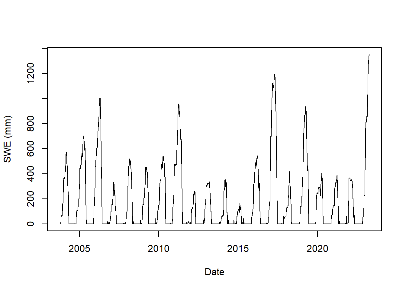

Figure 9.7: Snow water equivalent at SNOTEL site 1050.

Note the units are SI. If you download data directly from the SNOTEL web site the data would be in conventional US units. snotelr converts the data to SI units as it imports. The package includes a function snotel_metric that could be used to convert raw data downloaded from the SNOTEL website to SI units.

For this example, we will extract a single year, but set the dates to ensure the entire snow season is contained within a year. The snotel_phenology function makes this easy. By default it uses an offset of 180 days (so years begin 180 days before Jan 1) to accomplish this.

phenology <- snotelr::snotel_phenology(snow_data) # Key dates from the observed snow data
min(phenology$first_snow_acc)                     # Earliest snow accumulation in the record
#> [1] "2004-09-20"
max(phenology$last_snow_melt)                     # Latest snow melt in the record
#> [1] "2022-05-13"
mean(phenology$max_swe)                           # The mean of peak SWE for each year, mm
#> [1] 550.6222

Based on this, for this site we’ll subset the data using 1-Sep to 31-Aug to be sure an entire winter is in one year. In addition, create a data frame that only includes columns that are needed and only include a single year of data.

snow_data_subset <- subset(snow_data, as.Date(date) >= as.Date("2008-09-01") &
 as.Date(date) <= as.Date("2009-08-31"))
snow_data_sel <- subset(snow_data_subset, select=c("date", "snow_water_equivalent", "precipitation", "temperature_mean", "temperature_min", "temperature_max"))
plot(as.Date(snow_data_sel$date),snow_data_sel$snow_water_equivalent,
     type = "l",xlab = "Date", ylab = "SWE (mm)")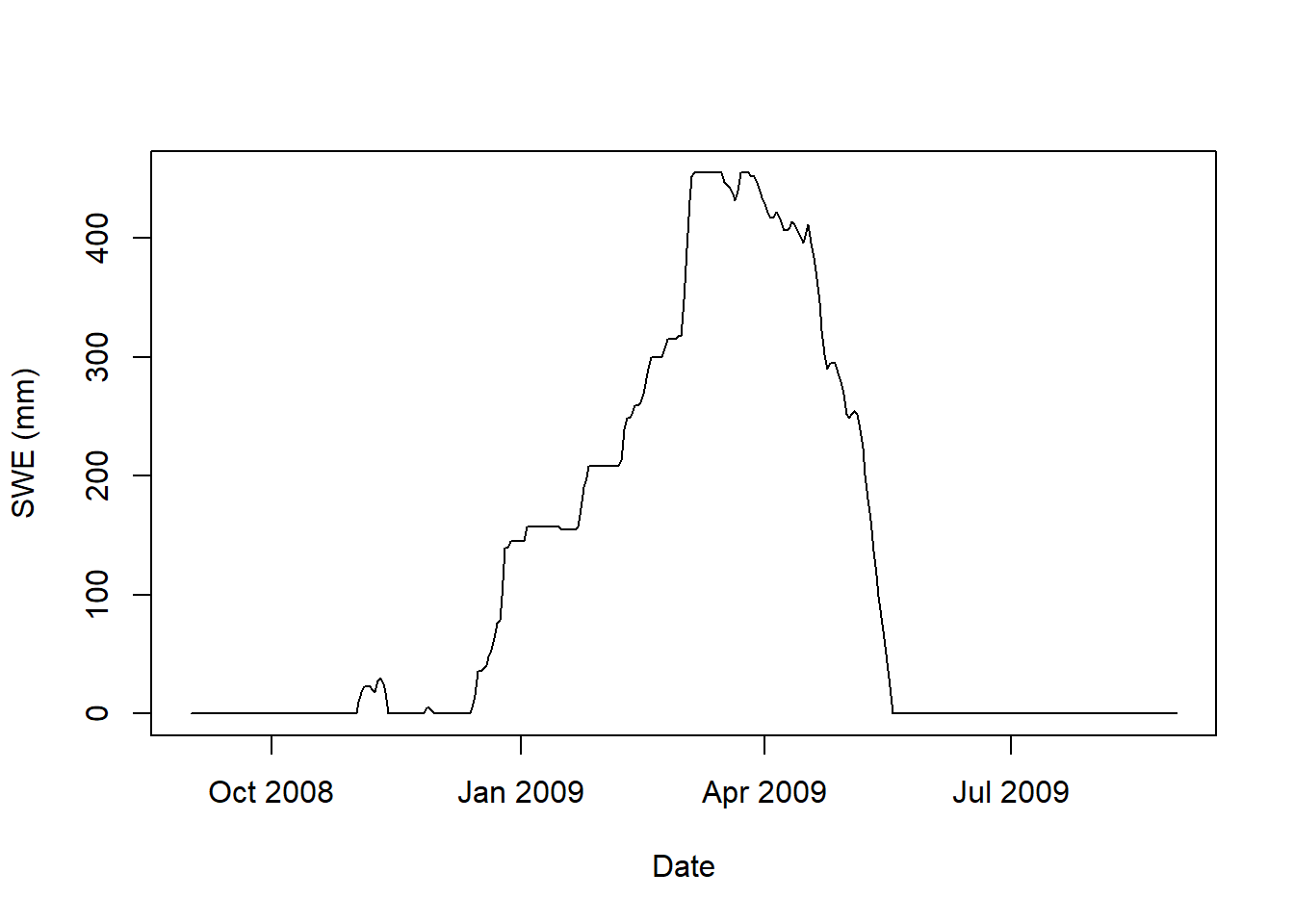

Figure 9.8: Snow water equivalent at SNOTEL site 1050 for Winter 2008-2009.

Now use a snow index model to simulate the SWE based on temperature and precipitation. The model used here is a modified version of that used in the hydromad package. The snow.sim command is used to run a snow index model; type ?hydromisc::snow.sim for details on its use. As a summary, the four main parameters you can adjust in the calibration of the model are:

The maximum air temperature for snow, Tmax. Snow can fall at air temperatures above as high as about 3\(^\circ\)C, but Tmax is usually lower.
The minimum air temperature for rain, Tmin. Rain can fall when near surface air temperatures are below freezing. This may be as low as -1\(^\circ\)C or maybe just a little lower, and as high as 1\(^\circ\)C (though higher than this can be justified in some cases).
Base temperature, Tmelt, the temperature at which melt begins. Usually the default of 0\(^\circ\)C is used, but some adjustment (generally between -2 and 2\(^\circ\)C) can be applied to improve model calibration.
Snow Melt (Degree-Day) Factor, kd, which describes the melting of the snow when temperatures are above freezing. Be careful using values from different references as these are dependent on units. Typical values are between 1 and 5 mm/d/\(^\circ\)C.

Two additional parameters are optional; their effects are typically small.

Degree-Day Factor for freezing, kf, of liquid water in the snow pack when temperatures are below freezing. By default it is set to 1\(^\circ\)C/mm/day, and may vary from 0 to 2 \(^\circ\)C/mm/day.
Snow water retention factor, rcap. When snow melts some of it can be retained via capillarity in the snow pack. It can re-freeze or drain out. This is expressed as a fraction of the snow pack that is frozen. The default is 2.5% (rcap = 0.025).

Start with some assumed values and run the snow model.

Tmax_snow <- 3  
Tmin_rain <- 2
kd <- 1
Tbase <- 0
snow_estim <- hydromisc::snow.sim(DATA = snow_data_sel, 
                                  Tmax = Tmax_snow, 
                                  Tmin = Tmin_rain,
                                  kd = kd,
                                  Tmelt = Tbase)

Now the simulated values can be compared to the observations. If not installed already, install the hydroGOF package, which has some useful functions for evaluating how well modeled output fits observations. In the plot that follows we specify three measures of goodness-of-fit:

Mean Absolute Error (MAE)
Percent Bias (PBIAS)
Root Mean Square Error (RMSE) or RMSE divided by the Standard Deviation (RSR)

These are discussed in detail in other references, but the aim is to calibrate (change the input parameters) until these values are low.

obs <- snow_data_sel$snow_water_equivalent
sim <- snow_estim$swe_simulated
hydroGOF::ggof(sim, obs, na.rm = TRUE, dates=snow_data_sel$date,
               gofs=c("MAE", "RMSE", "PBIAS"),
               xlab = "", ylab="SWE, mm", 
               tick.tstep="months", cex=c(0,0),lwd=c(2,2))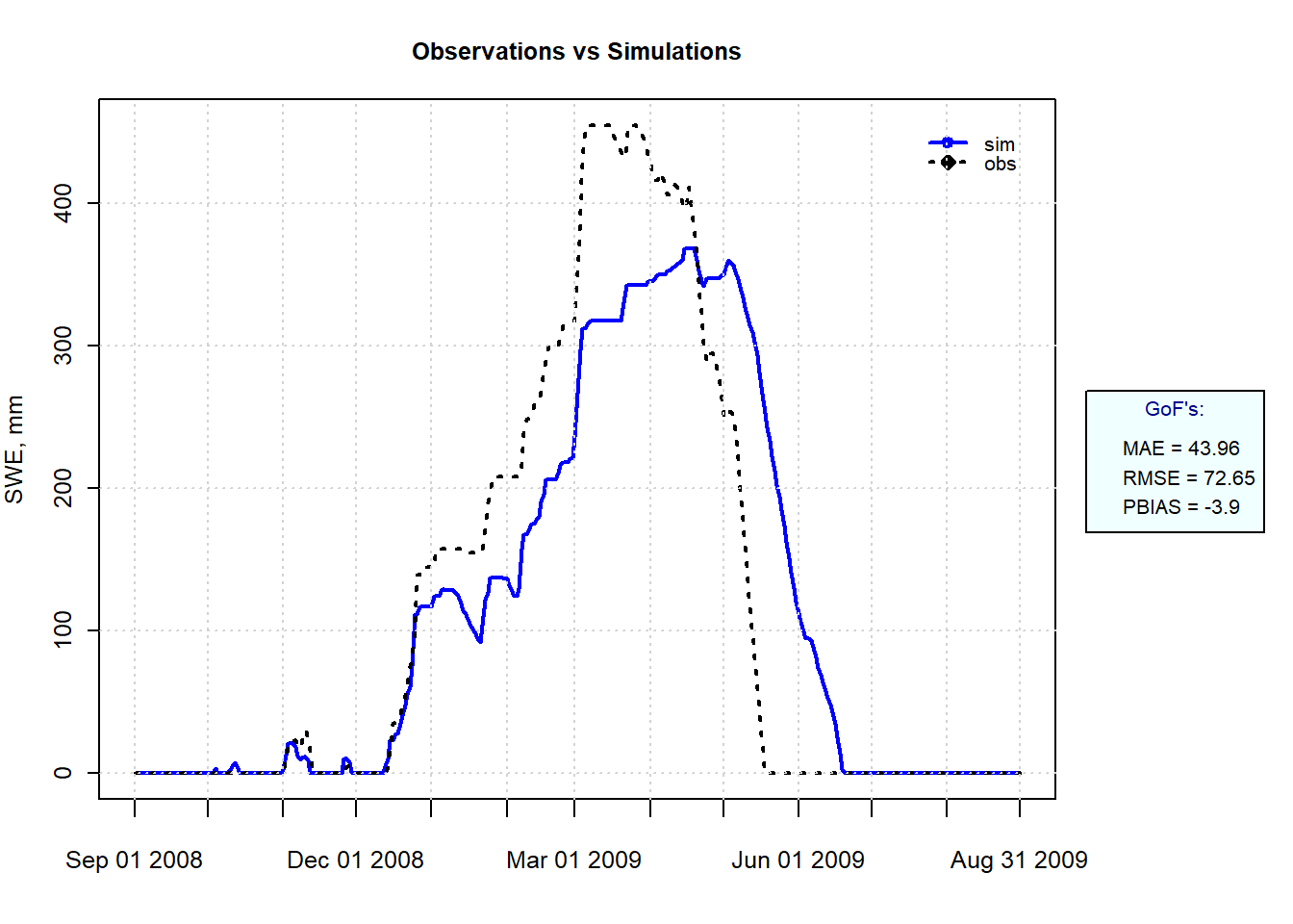

Figure 9.9: Simulated and Observed SWE at SNOTEL site 1050 for Winter 2008-2009.

Melt is overestimated in the early part of the year and underestimated during the melt season, showing why a single index is not a very robust model. Applying two kd values, one for early to mid snow season and another for later snowmelt could improve the model, but it would make it less useful for using the model in other situations such as increased temperatures.

9.4.3 Snow model calibration

While manual model calibration can improve the fit, a more complete calibration involves optimization methods that search the parameter space for the optimal combination of parameter values. The R function optim, part of the stats package installed with base R, is efficient at finding a local minimum or maximum to a function. For most hydrologic models finding the global optimum means searching the entire parameter space, since many local minima and maxima usually exist. Some version of Monte Carlo methods are used to do this.

There are many R packages to perform different variations of Monte Carlo simulations, but a simple implementation can be done manually using the foreach package. In this example the four main model parameters are each varied over 10 evenly spaced values, producing \(10^4\) unique parameters sets that need to be run. For each run, the function will return a value for RMSE.

# package needed for efficiently looping through all simulations
library(foreach)

# Create the sets of values of each parameter within a defined range
p_Tmax <- seq(-1, 3, length.out = 10)
p_Tmin <- seq(-1, 2, length.out = 10)
p_kd <- seq(0.5, 5, length.out = 10)
p_Tbase <- seq(-2, 2, length.out = 10)

# Assemble them into a data frame with all parameter combinations
p_all <- expand.grid(Tmax = p_Tmax, Tmin = p_Tmin, kd = p_kd, Tmelt = p_Tbase)

# Define the function to return a single test statistic for each simulation
fcn <- function(datain, Tmax, Tmin, kd, Tmelt){
  snow_estim <- hydromisc::snow.sim(DATA=datain, Tmax=Tmax, Tmin=Tmin, kd=kd, Tmelt=Tmelt)
  calib.stats <- suppressWarnings(hydroGOF::gof(snow_estim$swe_simulated,obs,na.rm=TRUE))
  return(as.numeric(calib.stats['RMSE',]))
}

Now the function needs to be used to run the snow model for every parameters combination. What is shown below is how to do this using the foreach package in a brute force manner, running all simulations on a single CPU. This takes a while.

out <- foreach(i = 1:nrow(p_all), .combine='c') %do% {
  fcn(snow_data_sel, p_all[i, "Tmax"], p_all[i, "Tmin"], p_all[i, "kd"], p_all[i, "Tmelt"])
}

Because the number of simulations can become very large, this command could be adapted to run the simulations in parallel using multiple cores by using the R package doParallel, which loads the parallel package (part of the base R installation). By running the foreach simulations with multiple processes, the run time using 7 of 8 available cores dropped from 5.9 minutes for a single CPU to 1.1 minutes. Aside from setting up the cluster before the command and stopping it after (essential for freeing up resources), the only change is the use of %dopar% instead of %do%.

library(doParallel)  
no_cores <- detectCores() - 1  
registerDoParallel(cores=no_cores)  
cl <- makeCluster(no_cores, type="PSOCK")  # On mac or linux you can change type to "FORK"
out <- foreach(i = 1:nrow(p_all), .combine='c') %dopar% {
  fcn(snow_data_sel, p_all[i, "Tmax"], p_all[i, "Tmin"], p_all[i, "kd"], p_all[i, "Tmelt"])
}
stopCluster(cl)

It can be helpful to look at the four parameters for the simulations that had the lowest RMSE. This presumes the tidyverse package has been installed.

# Combine results with parameters, sort by RMSE (ascending) 
out_all <- cbind(p_all, RMSE=out) |>  dplyr::arrange(RMSE)

library(ggplot2)
# Plot the parameters for the 10 best runs
dplyr::slice(out_all, 1:10) |> 
  tidyr::pivot_longer(-RMSE, names_to = 'param', values_to = 'value') |>
  ggplot(aes(x = RMSE, y = value)) + 
  geom_point() +
  facet_wrap(vars(param), scales = "free")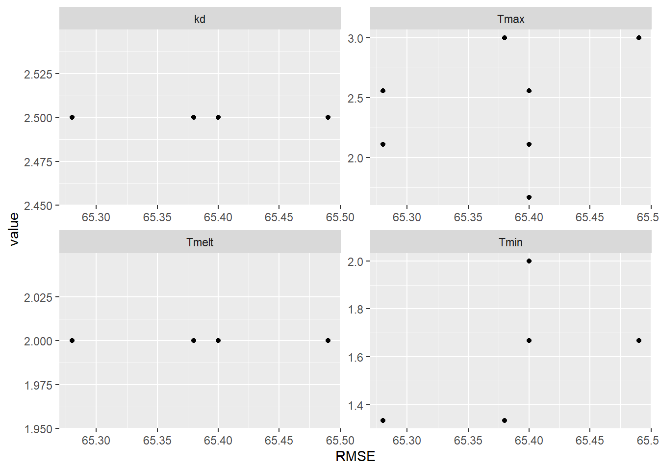

Figure 9.10: Parameter values for the 10 simulations with the lowest RMSE.

There are several occurrences of equal RMSE values, so some points are superimposed on one another. Some parameter values are consistent for all of the 10 best simulations: kd is 2.5 and Tmelt is 2\(^\circ\)C, but optimal values can be achieved with a variety of different combinations of Tmax and Tmin. The results using the optimal parameters can be plotted to visualize the simulation.

Tmax_opt <- max(out_all$Tmax[1],out_all$Tmin[1])
Tmin_opt <- min(out_all$Tmax[1],out_all$Tmin[1])
kd_opt <- out_all$kd[1]
Tmelt_opt <- out_all$Tmelt[1]

snow_estim_opt <- hydromisc::snow.sim(DATA=snow_data_sel,Tmax=Tmax_opt, 
                                      Tmin=Tmin_opt, kd=kd_opt, Tmelt=Tmelt_opt)
sim_opt <- snow_estim_opt$swe_simulated
hydroGOF::ggof(sim_opt, obs, na.rm = TRUE, dates=snow_data_sel$date,
               gofs=c("MAE", "RMSE", "PBIAS"),
               xlab = "", ylab="SWE, mm", 
               tick.tstep="months", cex=c(0,0),lwd=c(2,2))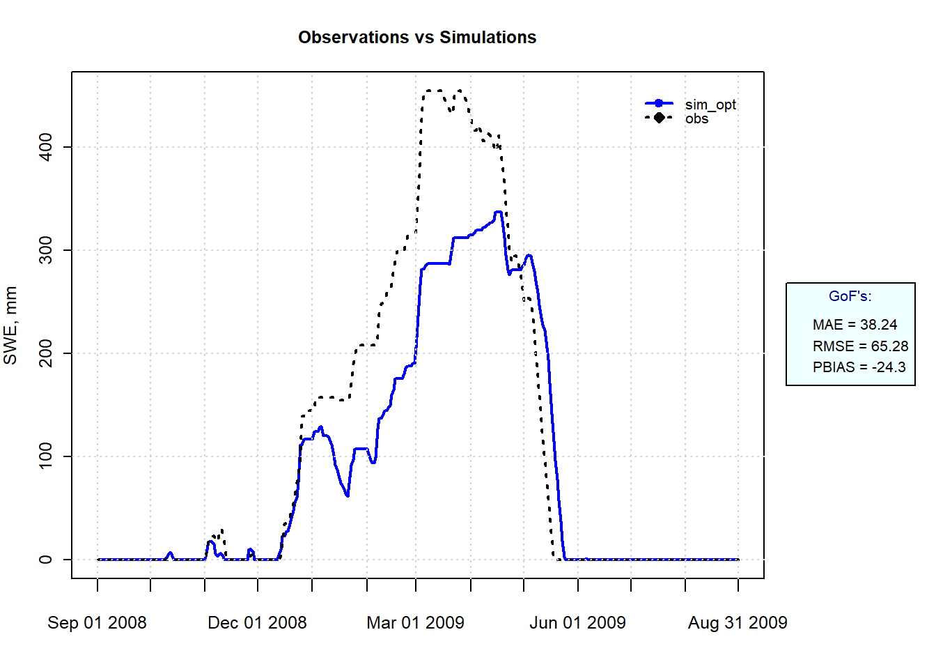

Figure 9.11: Simulated and Observed SWE at SNOTEL site 1050 for Winter 2008-2009 using the parameter set producing the lowest RMSE.

It is clear that a simple temperature index model cannot capture the snow dynamics at this location, especially during the winter when melt is significantly overestimated.

9.4.4 Estimating climate change impacts on snow

Once a reasonable calibration is obtained, the effect of increasing temperatures on SWE can be simulated by including the deltaT argument in the hydromisc::snow.sim command. Here a 3\(^\circ\)C uniform temperature increase is imposed on the optimal parameterization above.

dT <- 3.0 
snow_plus3 <- hydromisc::snow.sim(DATA=snow_data_sel,
                      Tmax=Tmax_opt, Tmin=Tmin_opt, kd=kd_opt, Tmelt=Tmelt_opt,
                      deltaT = dT)
simplusdT <- snow_plus3$swe_simulated
# plot the results
dTlegend  <- expression("Simulated"*+3~degree*C)
plot(as.Date(snow_data_sel$date),obs,type = "l",xlab = "", ylab = "SWE (mm)")
lines(as.Date(snow_estim$date),sim_opt,lty=2,col="blue")
lines(as.Date(snow_estim$date),simplusdT,lty=3,col="red")
legend("topright", legend = c("Observed", "Simulated",dTlegend),
       lty = c(1,2,3), col=c("black","blue","red"))
grid()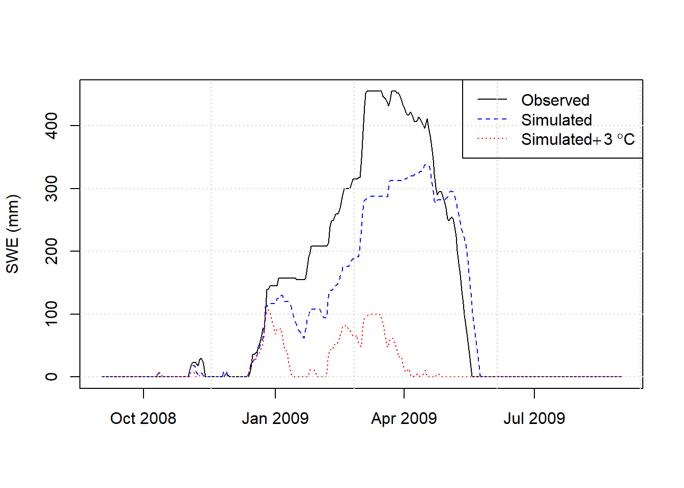

Figure 9.12: Observed SWE and simulated with observed meteorology and increased temperatures.

9.5 Watershed analysis

Whether precipitation falls as rain or snow, how much is absorbed by plants, consumed by evapotranspiration, and what is left to become runoff, is all determined by watershed characteristics. This can include:

Watershed area
Slope of terrain
Elevation variability (a hypsometric curve)
Soil types
Land cover

Collecting this information begins with obtaining a digital elevation model for an area, identifying any key point or points on a stream (a watershed outlet), and then delineating the area that drains to that point. This process of watershed delineation is often done with GIS software like ArcGIS or QGIS. The R package WhiteboxTools provides capabilities for advanced terrain analysis in R.

Demonstrations of the use of these tools for a watershed are in the online book Hydroinformatics at VT by JP Gannon. In particular, the chapters on mapping a stream network and delineating a watershed are excellent resources for exploring these capabilities in R.

For watersheds in the U.S., watersheds, stream networks, and attributes of both can be obtained and viewed using nhdplusTools. Land cover and soil information can be obtained using the FedData package.