Chapter 13 Groundwater
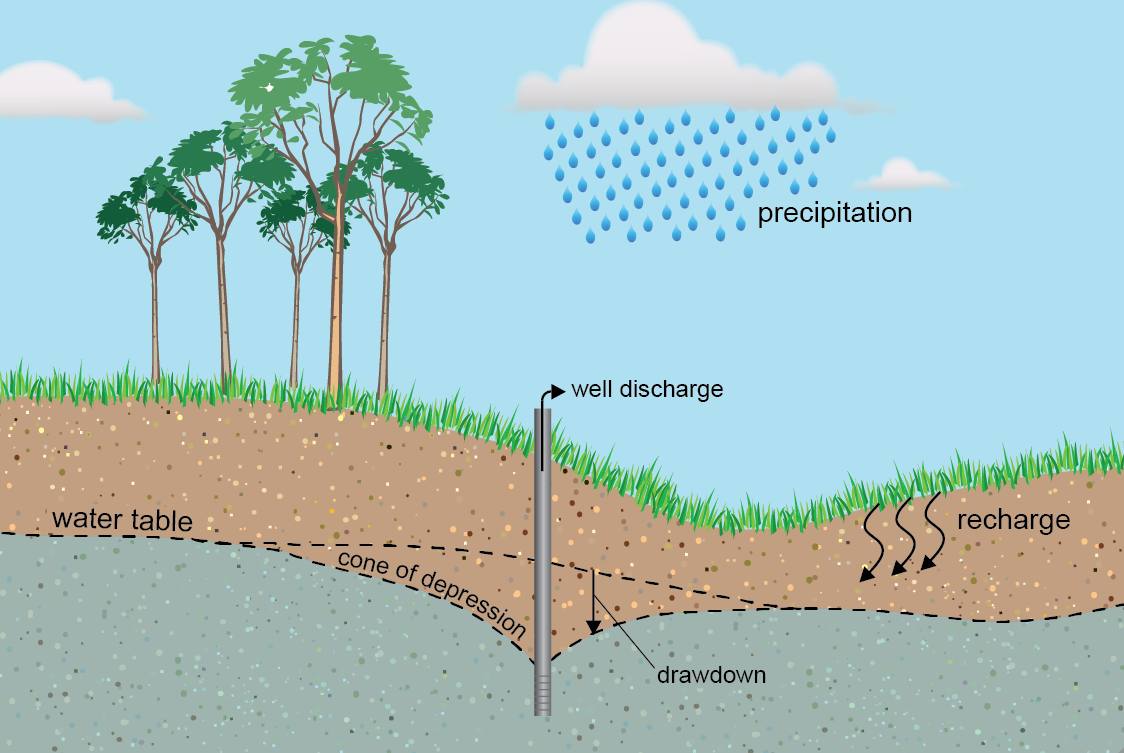
Figure 13.1: A conceptual aquifer with a pumping well U.S. Geological survey
Groundwater constitutes about 30% of the global freshwater reserves and is also under threat of depletion in many areas due to excessive extraction, mainly for irrigation (Gleeson et al., 2020). While in-depth methods for groundwater analysis will not be covered here, a few examples of using R in groundwater work are included here.
An excellent resource for introductory groundwater hydrology is USGS Water Supply Paper 2220 (Heath, 2004), which is freely available from the USGS.
The hydromisc package will need to be installed to access some of the code and data used below. If it is not installed, do so following the instructions on the github site for the package. In particular, portions of R packages rhytool and the defunct geotech have been wrapped into hydromisc.
13.1 Soil characteristics
Aquifers are deposits of soil or rock that are capable of allowing groundwater to flow. characterizing the soils, usually via soil texture, is one way to estimate important properties of aquifer material, like porosity (important for estimating the capacity to store water) and saturated hydraulic conductivity (how readily groundwater can move in an aquifer). This was discussed in the section on infiltration, which included the fundamental equation of Darcy’s law that governs the flow of fluid through a porous medium Equation (9.1).
One way to characterize aquifer material is using a sieve analysis. This allows the separation of soil into gravel, sand, silt, and clay, which can then be mapped onto a soil texture triangle to determine the soil texture using the USDA soil texture triangle, Figure 13.2.
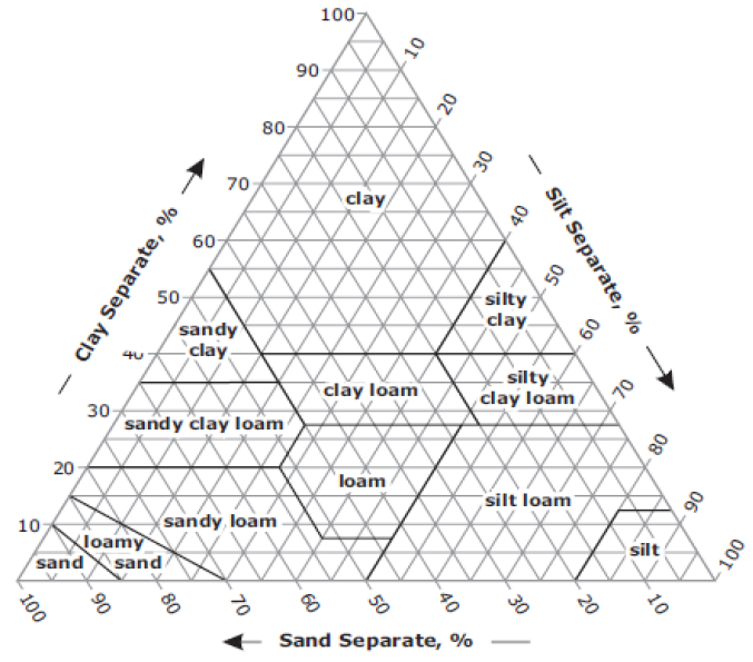
Figure 13.2: Soil texture triangle (USDA)
The soil texture is then used with something like Figure 9.3 to estimate soil hydraulic characteristics.
Other useful characterizations are the effective size of a given sample, D10, (D10 is the particle size where 10% of the particles are finer). The Coefficient of uniformity, Cu, is defined as \[Cu = D60/D10\] where D60 is the diameter for which 60 percent of the sample is finer.
Gravel (coarser than 4.75 mm, or a No.4 sieve), sand (4.75 mm > diameter > 0.075 mm or a No.200 sieve), silt (0.075 mm > diameter > 0.005 mm) and clay (finer than 0.005 mm) are defined under the USCS standard (ASTM 422-63 and ASTM D2487-92). The portions of a sample that are gravel, sand, and fines (silt and clay) are useful to quantify. If gravel is excluded, the components of sand, silt, and clay allow direct use of the soil texture triangle.
Example 13.1 A sieve analysis of a soil sample has a grain size distribution Table 13.1. Calculate the coefficient of uniformity for the portion finer than gravel, and the percent sand, silt, and clay (excluding gravel). Finally, determine the soil texture.
| % Finer | Diam, mm |
|---|---|
| 100 | 50.000 |
| 95 | 19.000 |
| 90 | 9.500 |
| 84 | 4.750 |
| 75 | 2.000 |
| 64 | 0.420 |
| 42 | 0.075 |
| 20 | 0.020 |
| 7 | 0.005 |
| 2 | 0.002 |
First input the data and create a grain size distribution plot to visualize the data.
df <- data.frame(
  sizes = c(50, 19, 9.5, 4.75, 2, .42, .075, 0.02, .005, .002),
  pct.finer = c(100,95,90,84,75,64,42,20,7,2))
hydromisc::grainSize.plot(size = df$sizes, percent = df$pct.finer)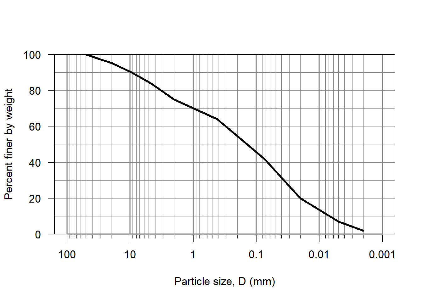
Figure 13.3: A grainsize distribution plot for the sample data.
Create a new data frame that only includes the portion finer than gravel.
df.ssc <- dplyr::filter(df, sizes <= 4.75) |>
  dplyr::mutate(pct.finer_ssc = 100*pct.finer/pct.finer[1])
To interpolate in a semi-log space to find D10 and D60 using the approx function, take the log of the sizes first, interpolate the value, then take the anti-log.
D10 <- 10^approx(x = df.ssc$pct.finer_ssc, y = log10(df.ssc$sizes), xout = 10)$y
D60 <- 10^approx(x = df.ssc$pct.finer_ssc, y = log10(df.ssc$sizes), xout = 60)$y
Cu <- D60/D10
These functions are also included in the hydromisc package.
as.data.frame(hydromisc::grainSize.coefs(size = df.ssc$sizes, percent = df.ssc$pct.finer_ssc))
#>         Cu        Cc         D10
#> 1 24.94169 0.8889553 0.005805067
To interpolate in a semi-log space to find the percent finer associated with a given diameter, a similar approximation function is applied as for D10 and D60, but with x and y reversed.For example, to find the percent finer than D = 0.05 mm:
This could be adapted to find the percent finer than the diameters of sand, silt, and clay. There is a built-in function for that.
pct_ssc <- hydromisc::percentSSC(size = df.ssc$sizes, percent = df.ssc$pct.finer_ssc)
as.data.frame(pct_ssc)
#>   psand psilt pclay
#> 1    50  41.7  8.33
A soil texture triangle can be plotted using the soiltexture package.
df.soiltextplot <- data.frame(SAND=pct_ssc$psand, SILT=pct_ssc$psilt, CLAY=pct_ssc$pclay)
soiltexture::TT.plot(class.sys="USDA.TT",
                     class.p.bg.col = T,
                     tri.data = df.soiltextplot,
                     cex.axis = 0.8, cex.lab = 0.9, main = "")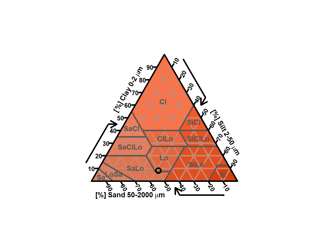
Figure 13.4: Soil texture triangle with example data plotted as a circle.
The soil texture for this example, a loam (near the sandy loam boundary), can be used with Figure 9.3 to estimate saturated hydraulic conductivity of the soil as approximately 1.3 cm/hr. Values determined in this way are subject to large uncertainty but can be a reasonable order of magnitude estimate.
Saturated hydraulic conductivity can also be measured through laboratory permeability tests or pumping tests in the field.
13.2 Hydraulic gradient and flow direction
To recap what was presented in the section on infiltration, the fundamental equation governing groundwater flow rate is Darcy’s law, Equation (13.1). Here the variables used are changed to be more consistent with the USGS. \[\begin{equation} q~=~ -K\frac{\partial h}{\partial L} \tag{13.1} \end{equation}\] where q is the flow of water per unit area (L/T), K is the hydraulic conductivity (L/T), H is the hydraulic head (L) and L is the distance along a flow path. Figure 13.5 shows the hydraulic gradient for a confined aquifer.
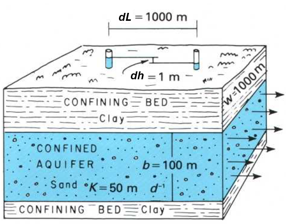
Figure 13.5: Hydraulic gradient in a confined aquifer (Heath, 2004). Note the dh term is measured in the direction of flow.
While in 1-D idealization like Figure 13.5 flow direction is clear, in the field the flow direction varies spatially and requires many observations and/or modeling to estimate. The USGS reference (Heath, 2004) illustrates a simple way to manually determine groundwater flow direction given water table elevations at three points. While a useful demonstration of interpolation methods, in practice many observations or estimations of groundwater levels are needed to describe the flow directions of groundwater in an aquifer. This standard method involves interpolating observations onto a regular grid and then creating contours based on the interpolated groundwater elevations.
Groundwater observations can be obtained from many sources. National scale data for the U.S. is available from the USGS, State of California data from the DWR (through its CASGEM program), and regional data are summarized by many local agencies.
The following demonstration uses a sample data set of groundwater elevations, all recorded in June 2020 in Santa Clara County, CA, included in the hydromisc package to produce contours of groundwater elevation and to infer flow directions.
13.2.1 Importing and transforming point data
Import the data from the hydromisc package. This was obtained from Valley Water, the agency serves as the regional Groundwater Sustainability Agency for California Sustainable Groundwater Management Act (SGMA). As part of its responsibilities under SGMA it manages and distributes data to promote local, sustainable groundwater management. The data have been extracted for a subset of wells and dates and reformatted into a spreadsheet for this example.
# path to sample data
datafile <- system.file("extdata", "scc_well_obs_202006.xlsx", package="hydromisc")
df <- readxl::read_excel(datafile)
head(df)
#> # A tibble: 6 × 6
#>   Well_ID    Lat   Lon Meas_Date           Depth_to_Water_ft Water_Lev_Elev_feet
#>   <chr>    <dbl> <dbl> <dttm>                          <dbl>               <dbl>
#> 1 06S01W2…  37.4 -122. 2020-06-15 00:00:00              4.61                31.4
#> 2 06S01W2…  37.4 -122. 2020-06-09 00:00:00            -28.6                 65.1
#> 3 06S01W3…  37.4 -122. 2020-06-15 00:00:00             33                   28.6
#> 4 06S01W3…  37.4 -122. 2020-06-15 00:00:00             10                   55.2
#> 5 06S01W3…  37.4 -122. 2020-06-09 00:00:00            -21.1                 64.7
#> 6 07S01W0…  37.4 -122. 2020-06-15 00:00:00             63                   23.0
It is helpful to view the data spatially, A couple of convenient R packages to use for working with this data are the sf (Simple Features, for spatial analysis) and mapview for easy interactive viewing of spatial data. First, make a spatial object out of the data frame, identifying latitude and longitude columns and then view it. The latitudes and longitudes are in the WGS84 coordinate system, designated as crs 4326.
gw_sf <- sf::st_as_sf(df, coords = c("Lon", "Lat"), crs = 4326)
mapview::mapview(gw_sf["Water_Lev_Elev_feet"],at=seq(20,80,10),layer.name="WS Elev, ft")
Before doing interpolation, note that the distance between the wells will be an important variable. Since right now the wells are defined by latitude and longitude, the distances would be in degrees, which are not useful for calculations. The data must be projected to a Cartesian coordinate system (x, y); a common one for California is UTM Zone 10N. Finding the crs (or epsg) code for any projection can be done using spatialreference.org. Here the WGS84/UTM Zone 10N is 32610. Transform the data to that with one command.
You can repeat the mapview command from above to verify that the locations haven’t changed, but now the dataframe has a geometry attribute with x and y coordinates (in meters).
13.2.2 Interpolating points to a regular grid (using kriging)
Kriging requires a mathematical representation of how the variability at one locations depends on other stations nearby. This is called a variogram (technically it is a semivariogram). This is calculated based on observations and the distances between the wells. Given n wells, there are \(n(n-1)/2\) pairs of wells. That means the 15 observations in this example create 105 pairs of points that can be used to fit a variogram model. More points is better.
A theoretical model (curve) is fit to the data, the shape of which is described by the sill, nugget, range, and model type (such as spherical). These terms are illustrated in Figure 13.6. Low values on the y-axis mean high correlation, so this diagram indicates close wells influence the value estimated at any unknown location, which intuitively makes sense.
Figure 13.6: A sample variogram U.S. Dept of Energy, PNNL
Now create a variogram from the observations and fit a theoretical model to that. The variogram function requires a formula. A formula object is created using the ~ operator, which separates names of dependent variables (to the left of the ~ symbol) and independent variables (to the right of the ~ symbol). Writing 1 to the right of the ~ symbol, as in ~ 1, means that there are no independent variables. This approach uses two packages: gstat to define the variogram, and automap to automate the optimal fit to the data. gstat can also fit variograms, but requires more input based on the user’s knowledge of kriging.
f.1 = as.formula("Water_Lev_Elev_feet ~ 1")
v = gstat::variogram(f.1, data = gw_sf_t )
vario.fit = automap::autofitVariogram(f.1, as(gw_sf_t,"Spatial") )
vario.fit$var_model
#>   model    psill    range
#> 1   Nug   0.0000    0.000
#> 2   Gau 312.0808 1183.641
The plot of the semivariogram illustrates the model fit to the observations.
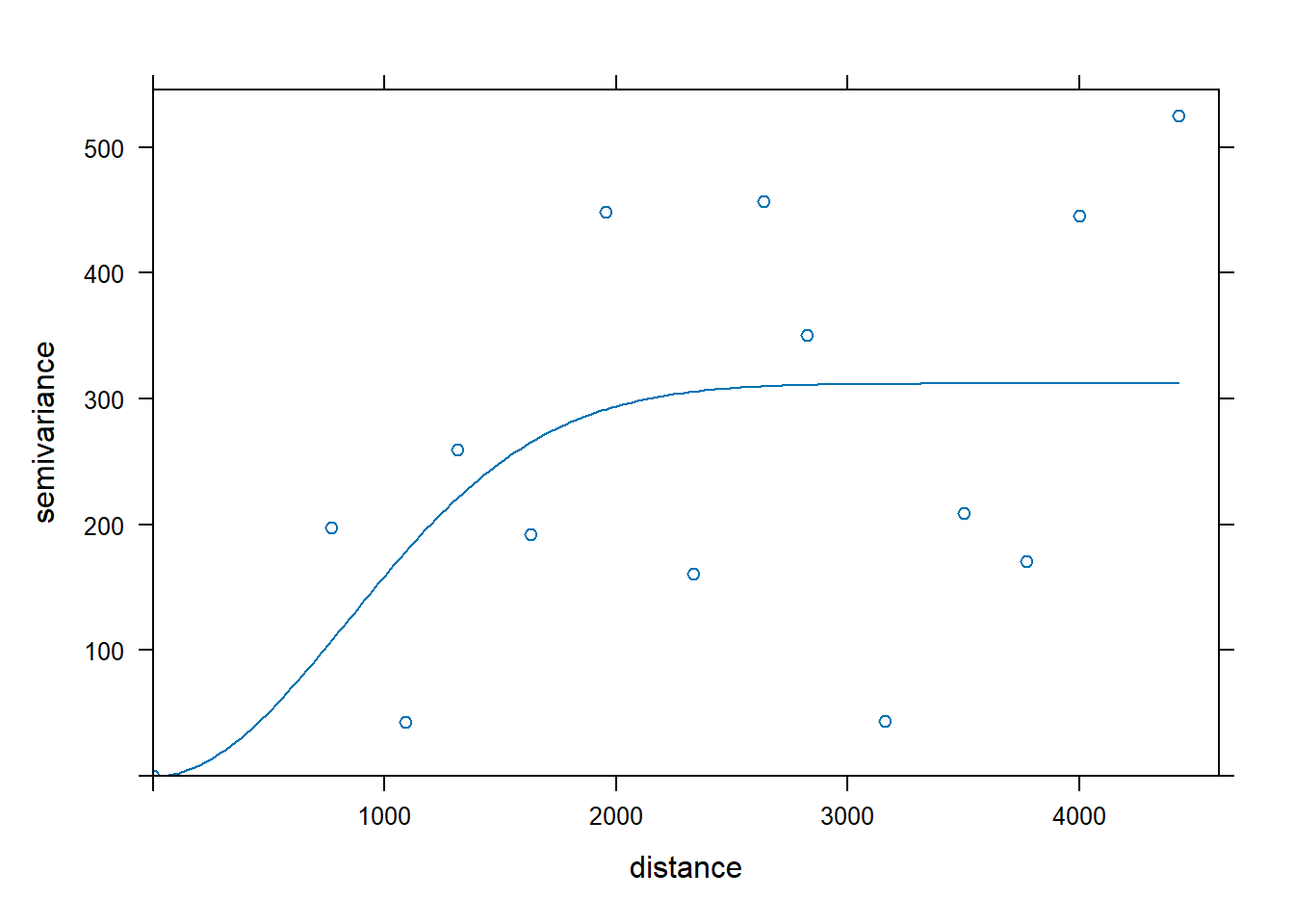
Figure 13.7: A variogram plotted for the sample data used in this example.
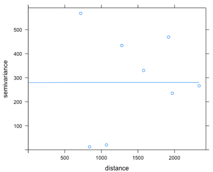
Figure 13.8: A variogram fit to the first 11 observation in the sample data
A horizontal variogram model is called a “pure nugget” indicating the data show no relation between the variable (groundwater elevation) and distance. This often happens if the distance between observations is small relative to the scale of spatial variability. Kriging is not helpful when this occurs; interpolation would just produce the mean value everywhere.
To begin interpolation, you first need to define the points to which you want interpolation done. The sf package has a function that makes this easy: generate a bounding box for the area of the original data, make a grid (here equally spaced at 500 m intervals).
outer_bound <- sf::st_make_grid(sf::st_bbox(gw_sf_t), n=1)
pts <- sf::st_make_grid(outer_bound, cellsize = 500, what = "centers", square = TRUE)
Applying the kriging model to interpolate to these grid points can be done in several ways. Here the autoKrige function in the automap package is used to fit the models to the data and generate new interpolated values onto the grid of defined points.
The gw_interpolated object contains a lot of information on the fitted model, the spatial variance, and the values predicted by kriging. For plotting interpolated values, it is convenient to create an sf object with that information, which can then be plotted.
gw_interp_sf <- sf::st_as_sf(gw_interpolated$krige_output)
mapview::mapview(gw_interp_sf, zcol = 'var1.pred', layer.name = "WS Elev, ft")
The last step is to turn the interpolated points into a raster so they can be plotted with contour lines. This example uses some basic functions of the terra package. First a spatial vector is defined from the pts layer, a raster is defined based on that (again with a spatial resolution of 500 m), and a new spatial raster is created. Checking the minimum and maximum values in the raster allows refined control of the colorbar when plotting.
v <- terra::vect(pts)
r <- terra::rast(v, res = 500)
gw_rast <- terra::rasterize(gw_interp_sf, r, 'var1.pred', fun = mean, na.rm=TRUE)
terra::minmax(gw_rast)
#>         mean
#> min 23.00131
#> max 74.01109
Using the values from the raster as a guide, a plot can be created using terra.
brks <- seq(20, 75, 5)
cols <- terrain.colors(length(brks)-1)
terra::plot(gw_rast, , type="continuous", breaks=brks, col=cols, reset = TRUE, axes = F)
terra::contour(gw_rast, add = TRUE)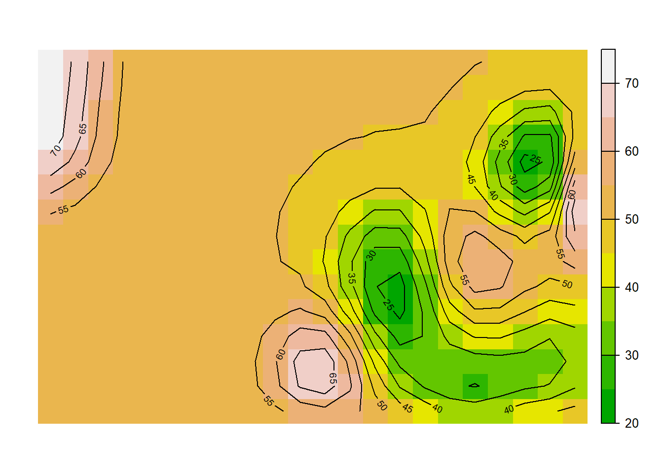
Figure 13.9: Contours of groundwater elevations in ft.
Many other mapping options are available, such as using sf to create a layer with the contours and then mapview to plot it. Sample code is shown here but output is not.
gw_contour = sf::st_contour(gs1_rast, breaks = b,contour_lines = TRUE)
m1 <- mapview::mapview(gs1_rast,at=b,col.regions=terrain.colors(length(b)-1),layer.name="WS Elev, ft")
m2 <- mapview::mapview(sf::st_geometry(gw_contour))
m1 + m2
Vector plots can also be created using the metr and ggplot2 packages.
13.3 Groundwater flow in aquifers
This section introduces the basic equations for groundwater flow and shows how they can be applied for confined and unconfined aquifers. The effect of pumping will be in the next section.
13.3.1 Fundamental equations
By combining equations for mass balance, Darcy’s law (Equation (13.1)), and relationships describing aquifer porosity and water and aquifer compressibility, a theoretical equation can be derived for the two idealized aquifer types: confined and unconfined. For groundwater flow in a 2-D, isotropic and homogeneous (so K is the same everywhere and in every direction) system these appear as Equations (13.2) and (13.3). \[\begin{equation} Confined: \frac{\partial^2 h}{\partial x^2}+\frac{\partial^2 h}{\partial y^2}=\frac{S}{T}\frac{\partial h}{\partial t} \tag{13.2} \end{equation}\] \[\begin{equation} Unconfined: \frac{\partial^2 h^2}{\partial x^2}+\frac{\partial^2 h^2}{\partial y^2}=\frac{2S_y}{K}\frac{\partial h}{\partial t}-\frac{2w}{K} \tag{13.3} \end{equation}\] where h is the hydraulic head at a point (equal to the piezometric surface height for a confined aquifer or the water table elevation for an unconfined one), S is the storativity, Sy is the specific yield and T is the transmissivity. These are illustrated in Figure 13.10.
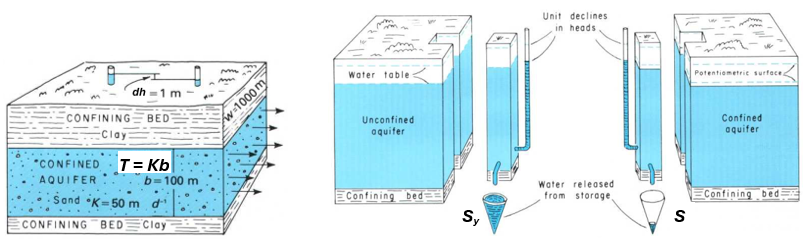
Figure 13.10: Transmissivity, storativity, and specific yield, adapted from (Heath, 2004).
A common simplification is applied to Equation (13.3) when the hydraulic gradient or drawdown is small relative to aquifer thickness (\(\partial h \ll h\) and \(h \approx b\)) so it becomes linearized like the confined solution in Equation (13.2). \[\begin{equation} Unconfined \left(\partial h \ll h\right): \frac{\partial^2 h}{\partial x^2}+\frac{\partial^2 h}{\partial y^2}=\frac{2S_y}{Kb}\frac{\partial h}{\partial t}-\frac{2w}{Kb} \tag{13.3} \end{equation}\]
13.3.2 Groundwater flow under steady state conditions
For a 1-D, homogeneous, isotropic aquifer, Equations (13.2) and (13.3) can be solved explicitly for steady state conditions. When combined with Darcy’s law (Equation (13.1)) relationships can be derived to solve for piezometric head (or water table height) for a given flow, Q (or flow per unit width, q’), or to solve for the flow given head values. This is illustrated in Figure 13.11.
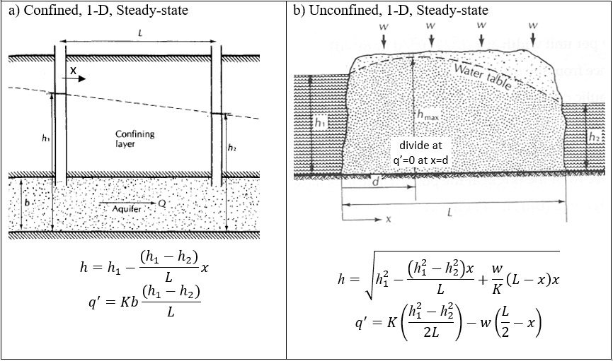
Figure 13.11: Steady-state solutions for flow in an isotropic, homogeneous aquifer. Figures adapted from (Fetter, 2001).
13.4 Drawdown due to pumping
When a well pumps water from an aquifer, the piezometric surface drops (for a confined aquifer) or the water table declines (for unconfined). This is illustrated in Figure 13.12.
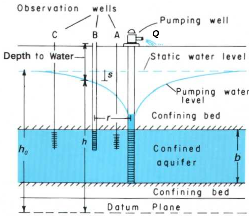
Figure 13.12: Drawdown in a pumping well in a confined aquifer (Heath, 2004).
The definitions illustrated in Figure 13.12 show the relationship between head, h, and drawdown, s, and how that varies with radial distance from a pumping well, r.
13.4.1 Steady state well drawdowns
As with flow in an aquifer under steady state conditions, analytical solutions make solving the groundwater flow equations straightforward. These equations can be solved for aquifer properties given pumping rate (Q) and observations of drawdown (or head), or the reverse. These are shown in Equations (13.4) and (13.5). \[\begin{equation} Confined: T=Kb=\frac{Q}{2\pi \left(h_2-h_1\right)}\ln\left(\frac{r_2}{r_1}\right)=\frac{Q}{2\pi \left(s_1-s_2\right)}\ln\left(\frac{r_2}{r_1}\right) \tag{13.4} \end{equation}\] \[\begin{equation} Unconfined: K=\frac{Q}{\pi \left({h_2}^2-{h_1}^2\right)}\ln \left(\frac{r_2}{r_1}\right) \tag{13.5} \end{equation}\]
Equations (13.4) and (13.5) can be rearranged to solve for flow given aquifer parameters. \[\begin{equation} Confined: Q=2\pi T\frac{h_2-h_1}{\ln \left(\frac{r_2}{r_1}\right)} \tag{13.6} \end{equation}\] \[\begin{equation} Unconfined: Q=\pi K\frac{{h_2}^2-{h_1}^2}{\ln \left(\frac{r_2}{r_1}\right)} \tag{13.7} \end{equation}\]
13.4.2 Time-varying well drawdowns
The much more common situation is for wells to be operated for discrete times, so the steady state solutions will not apply. The fundamental equation used to describe this is Equation (13.8) (Theis, C.V., 1935). \[\begin{equation} s=h_0-h=\frac{Q}{4\pi T}W(u) \tag{13.8} \end{equation}\] where W(u) is the well function (or exponential integral) of the Boltzman variable, \(u\), as in Equation (13.9). \[\begin{equation} u=\frac{r^2S}{4Tt} \tag{13.9} \end{equation}\] The \(W(u)\) function is often approximated by the (infinite) timeseries: \[\begin{equation} W(u)=-0.5772 - \ln(u) + u - \frac{u^2}{2 \cdot 2!} + \frac{u^3}{3 \cdot 3!} - \frac{u^4}{4 \cdot 4!} + ... \tag{13.10} \end{equation}\]
Methods to estimate drawdown at a given time are straightforward, while doing the reverse – estimating aquifer parameters given drawdown – are more complicated. Methods to do this manually are demonstrated in any groundwater hydrology text, such as (Heath, 2004). Some functions for this are included in the hydromisc package, which are shown in the examples below.
Read in some sample drawdown data from the hydromisc package. Use the list of times (recorded in minutes) in that file.
datafile <- system.file("extdata", "drawdowns.xlsx", package="hydromisc")
df_dd <- readxl::read_excel(datafile)
times <- df_dd$t_min
Supply the aquifer parameters (properties), which are known in this case. Convert the times from minutes to days. Using consistent units this these functions is essential!
To calculate the drawdown at each time for a single distance, 60 m from the pumping well in this case, for a pumping rate of 2500 m\(^3\)/d (about 460 gpm), the drawdown can be calculated as shown below. This approach uses the expint_E1 function of the expint package to calculate the W(u) in Equation (13.8) for all u values.
rs <- 60                          # distance in m
Q <- 2500                         # pumping rate in m^3/d
us <- (rs)^2*St/(4*Tr*t)          # Calculate all u values -- units must be consistent
Wus <- expint::expint_E1(us)      # find the W(u) for each u value
dds <- Q/(4*pi*Tr)*Wus            # calculate the drawdowns
plot(t, dds, log="xy", xlab="time, d", ylab="drawdown, m", type="l")
grid()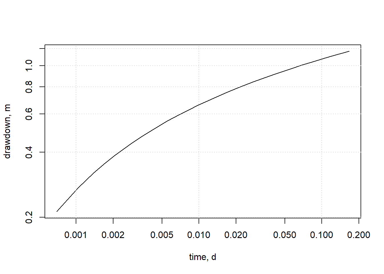
Figure 13.13: Drawdown at 60 m from pumping well.
Of course, a simple function could clean up R code when calculations are done many times. Because the drawdown data begin with zero values the expint function produces a warning about underflow, which is suppressed here.
drawdown <- function(t, Q, r, Tr, St) {
  if(length(t) > 1 && length(r) > 1) {
    stop("Either t or r must be of length 1.")
  }
  us <- (r)^2*St/(4*Tr*t)
  Wus <- suppressWarnings(expint::expint_E1(us))
  dds <- Q/(4*pi*Tr)*Wus
  return(dds)
}
Similarly, drawdowns can be calculated at many distances for a given time. The following example uses the function created above.
rs <- seq(from=1, to=100, by=5)
t1 <- 0.05
dds <- drawdown(t=t1, Q=Q, r=rs, Tr=Tr, St=St)
plot(rs, dds, xlab="distance from pumping well, m", ylab="drawdown, m", type="l")
grid()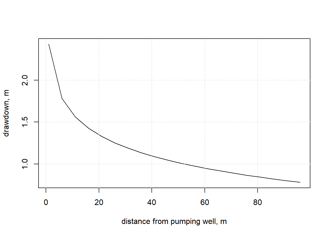
Figure 13.14: Drawdown at time=0.05 day (72 minutes) after pumping begins.
Drawdown due to multiple wells are additive, and can be positive (due to a pumping well) or negative (for a recharge well). For a well that is operated for a fixed time, a recharge well can be added at the same point but with a negative pumping rate that begins when the pump is turned off. That is demonstrated in the following example.
Example 13.2 Find the drawdown 200 ft from a pumping well that is operated for 6 hours at Q = 60 gpm (481.3 ft\(^3\)/h) and then turned off. Aquifer characteristics are St = 0.001 and Tr = 16.67 ft\(^2\)/h (based on K=5 ft/d and b = 80 ft).
Assign variables to aquifer parameters, pumping rate, distance, and a variety of times. Use the function above to calculate the drawdowns at all times and create a data frame of the results.
St <- 0.001
Tr <- 16.67
Q1 <- 481.3
r <- 200 #ft
times <- seq(from=0, to=16, by=0.25)   #times in hours
ddpump <- drawdown(t=times, Q=Q1, r=r, Tr=Tr, St=St)
df.ddpump <- data.frame(t=times, s=ddpump)
Now calculate the same drawdowns but for a recharge pump injecting water at the same rate as the initial one pumped, create another data frame and adjust the times to start 6 hours later.
ddrech <- drawdown(t=times, Q = -Q1, r=r, Tr=Tr, St=St)
df.ddrech <- data.frame(t=times+6, s=ddrech)
Now join the two data frames, aligning them by the time field. Since drawdown columns have the same name (‘s’) they are renamed in the combined data frame to ‘s.x’ and ‘s.y’. Times for the first 6 hours will have NA values after the join, and those are replaced by zeros, and a new column with total drawdown is added. A plot helps see the recovery of the well drawdown after the well is turned off.
total <- dplyr::left_join (df.ddpump, df.ddrech, by='t') |>
  tidyr::replace_na(list(s.y = 0)) |>
  dplyr::mutate(drawdown = s.x + s.y)
plot(total$t, total$drawdown, xlab="time, hr", ylab="drawdown, ft",
     xlim=range(times), type="l")
grid()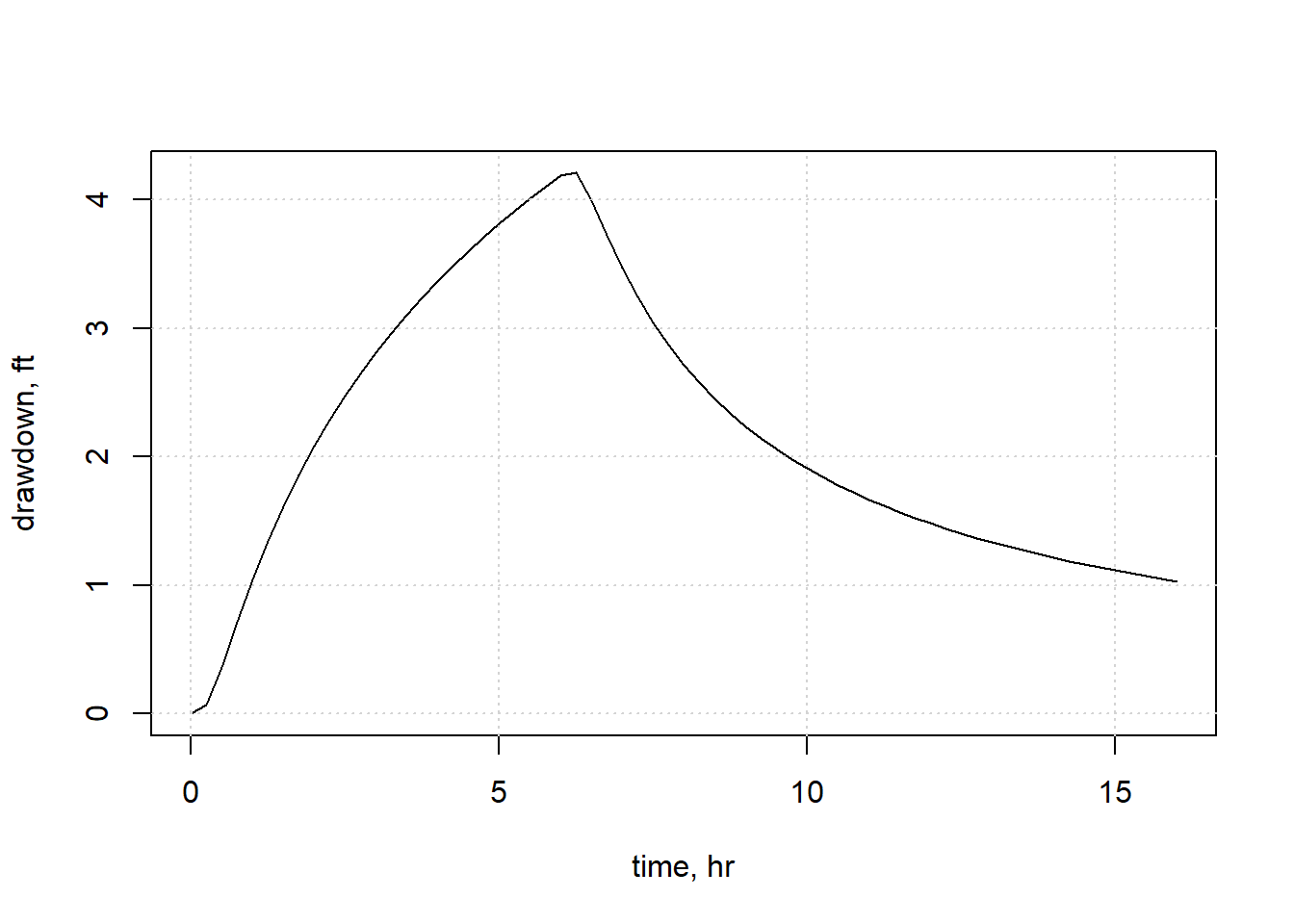
Figure 13.15: Drawdown for a well with pumping turned off at t=6 hours.
13.4.3 Boundaries near pumping wells
The theoretical equations for calculating drawdown assume infinite horizontal extent. In reality the drawdown due to pumping a well can be influenced by boundaries such as nearby rivers. These can be accommodated by including image wells, which are pumping (or recharge) wells that do not exist but can be used to simulate the effect of a river or impermeable boundary. Two common idealized boundaries are illustrated in Figure 13.16.
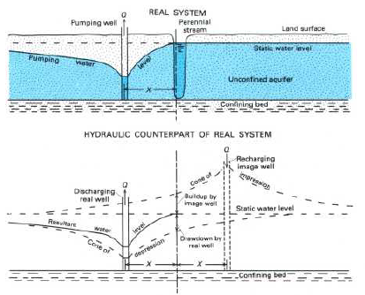
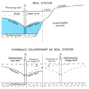
Figure 13.16: Two common types of boundaries and how they are represented in a groundwater flow analysis (Heath, 2004).
Including the effect of a boundary only requires including (by adding) the drawdown or recharge from the image well. The presence of a river (or other constant head boundary like a lake) will tend to lessen the drawdown; an impermeable boundary increases the drawdown.
When plotting drawdown data, the effect of these boundaries appears similar to Figure 13.17.
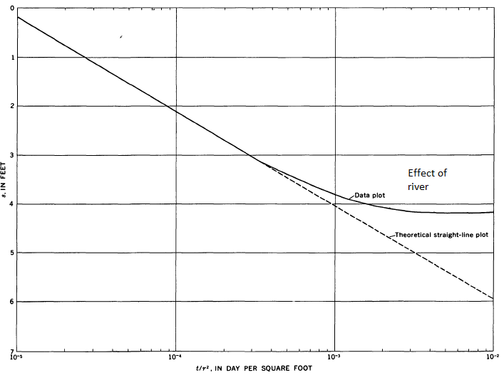
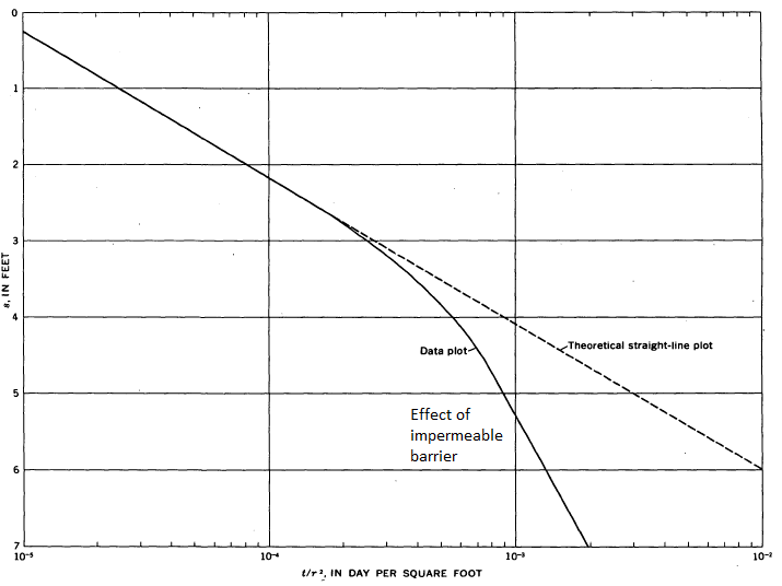
Figure 13.17: The effects of two common types of boundaries on time-drawdown plots. (Lohman, S.W., 1972).
13.4.4 Capture zones
As opposed to the above drawdowns, which all assumed a static, horizontal water table or piezometric surface, if the water table has a slope the flow patterns are more complex. One effect is that of a capture zone, where flow within it eventually will be drawn in by the well, and flow outside the capture zone continues downgradient. the is depicted in Figure 13.18.
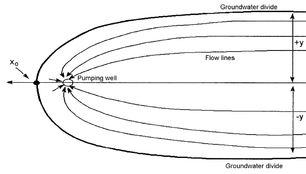
Figure 13.18: The capture zone is an aquifer with a gradient that slopes downward to the left. (U.S. Army Corps of Engineers, 1999).
The location of the capture zone (for a confined aquifer) is described by Equation (13.11). \[\begin{equation} x = \frac{-y}{\tan(2 \pi K b i y/Q)} \tag{13.11} \end{equation}\] The maximum value for y, as x \(\rightarrow\) \(\infty\) is \[\begin{equation} y_{max} = \frac{Q}{2Kbi} \tag{13.12} \end{equation}\] The location of the downgradient stagnation point is defined by \[\begin{equation} x_o = \frac{-Q}{2 \pi Kbi} \tag{13.13} \end{equation}\] where i is the regional piezometric gradient (\(\Delta h/\Delta L\)).
Example 13.3 A contamination source has been identified 90 ft from a pumping well, downgradient. With known aquifer properties K=1500 ft/d, i=0.3% and b=75ft, what pumping rate would be permissible (while keeping the contamination source outside the capture zone)?
Rearrange Equation (13.13) to solve for Q using \(x_o=-90\) ft.
K <- 1500   # ft/d
i <- 0.003  # gradient, unitless
b <- 75.    # ft
x0 <- -90    # ft
Q <- -2*pi*K*b*i*x0
cat(sprintf("Flow = %.0f ft%s/d", Q, '\u00B3'))
#> Flow = 190852 ft³/d
The complete capture zone can be determined as well.
capzone <- function(y) {
  -y/(tan(2*pi*K*b*i*y/Q))
}
ymax <- Q/(2*K*b*i)
y <- seq(from=-ymax*0.9, to=ymax*.9, length.out = 100)
x <- capzone(y)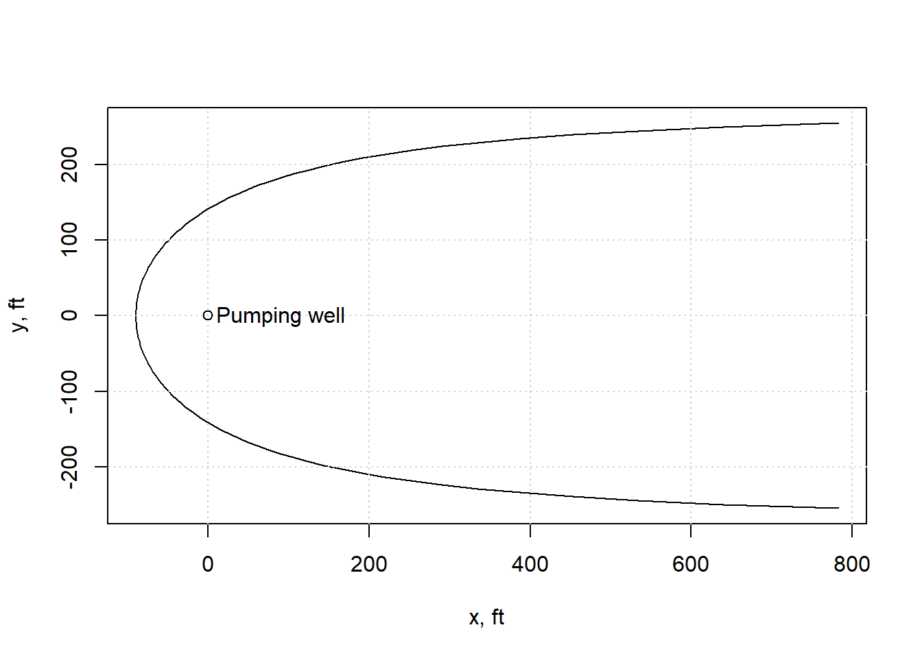
Figure 13.19: The capture zone for the example.
13.5 Determining aquifer characteristics from drawdown observations
If there is a complete set of drawdown observations at a set distance from a pumping well, values for storativity and transimissivity can be obtained using any equation solving technique. There are also graphical methods (Heath, 2004).
13.5.1 Cooper-Jacob approximation
When enough time has passed, or when \(u < 0.05\), the drawdown from a pumping well tends to plot linearly on a semi-logarithmic graph. When this is the case, the first two terms in Equation (13.10) dominate, and terms to the right can be neglected, which will plot as a straight line with drawdown plotted against the logarithm of time. The graphical procedure consists of:
- Plot drawdown, s, vs time on log-linear paper (time on the log scale).
- Fit a straight line to the linear portion of the drawdown data.
- Where the straight line intersects s=0, the corresponding time \(t_0\) is recorded.
- The difference in drawdowns, \(\Delta s\) at two times separated by one log cycle is recorded.
Transmissivity and Storativity are then calculated using Equations (13.14) and (13.15). \[\begin{equation} T=\frac{2.3 Q}{4\pi \Delta s} \tag{13.14} \end{equation}\] \[\begin{equation} S=\frac{2.25 T t_0}{r^2} \tag{13.15} \end{equation}\]
Example 13.4 Use the drawdown data imported above, measured 60 m from the pumping well, and use the same pumping rate of 2500 m\(^3\)/d. Estimate the storativity and transmissivity of the aquifer material using the Cooper-Jacob approximation.
Following the steps above, first plot the data to estimate the time after which the curve becomes linear.
plot(df_dd$t_min, df_dd$s_m, ylim = rev(range(df_dd$s_m)), xlim = c(0.1,300),
     xlab="time, min", ylab="drawdown, m", log = "x", pch = 1)
grid()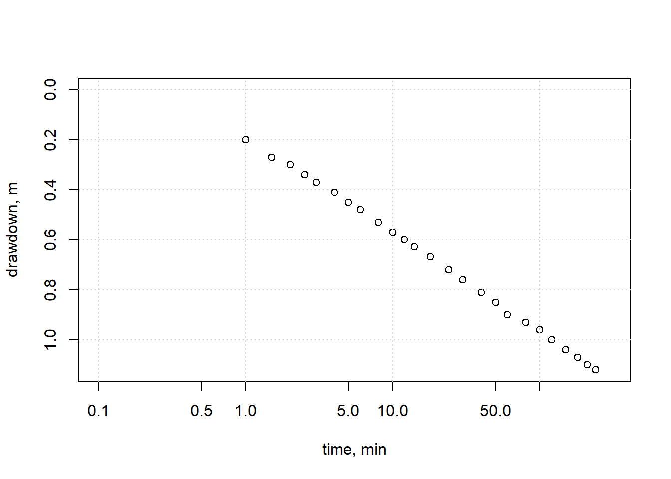
Figure 13.20: Observed drawdown vs. time.
From Figure 13.20 the relationship appears linear (in semi-log space) after time \(\approx\) 4 min. The data will be subset to times later than that, and a straight line fit to that subset. Note that x is the base-10 logarithm of time.
df_dd_linear <- dplyr::filter(df_dd, t_min > 4)
x <- log10(df_dd_linear$t_min)
y <- df_dd_linear$s_m
lf <- lm(y ~ x)
Now \(t_0\) and \(\Delta s\) can be estimated. Note that time is transformed back from base-10 logarithm.
t0 <- 10^(-coef(lf)[[1]]/coef(lf)[[2]])
s_logcycle <- predict(lf, data.frame(x=c(log10(10), log10(100))))
delta_s <- s_logcycle[[2]] - s_logcycle[[1]]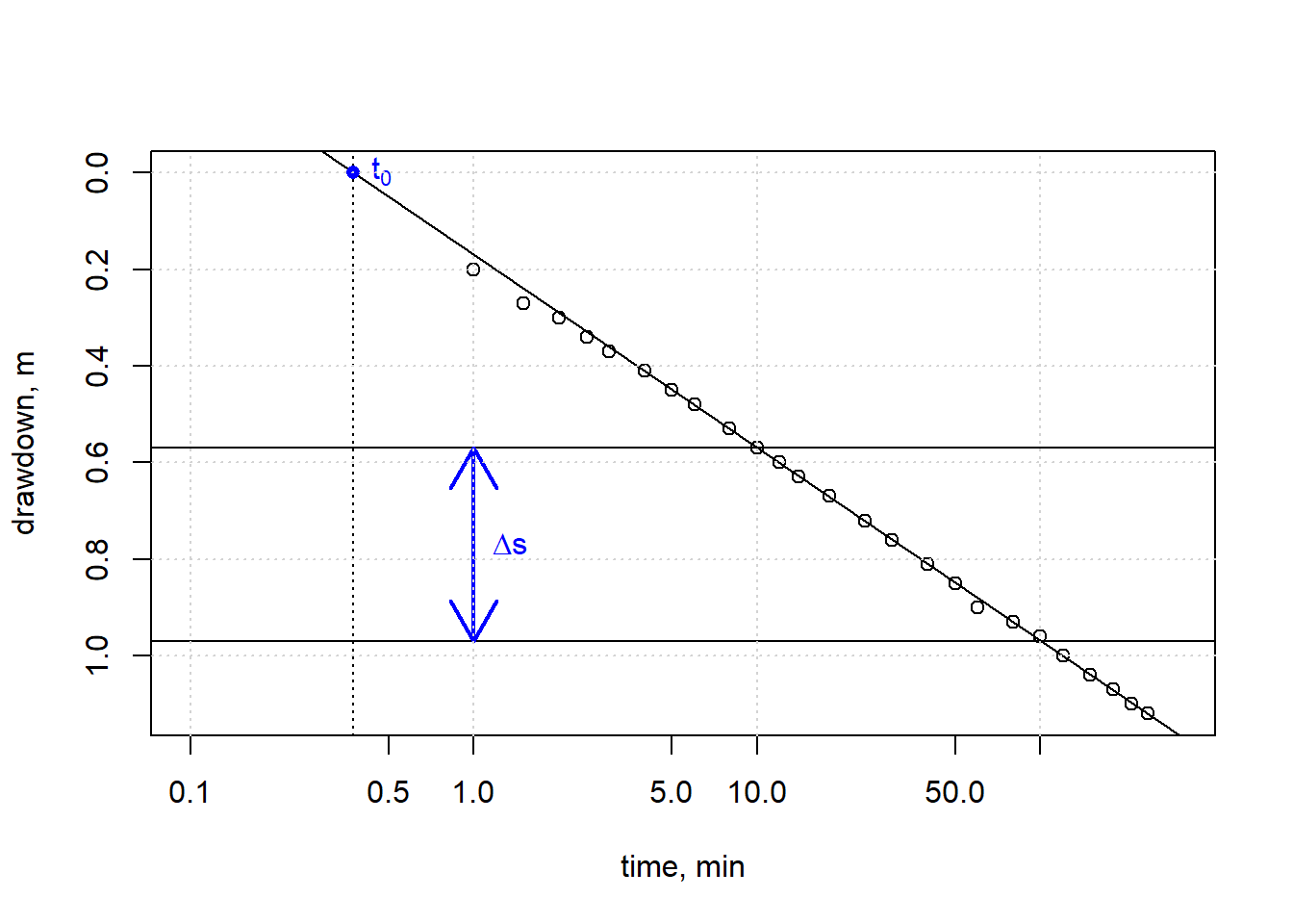
Figure 13.21: Observed drawdown vs. time illustrating the Cooper-Jacob calculations.
Finally, the known information is used to calculate \(T\) and \(S\) using Equations (13.14) and (13.15).
Q <- 2500  # m3/d
r <- 60
Tr <- 2.3*Q/(4*pi*delta_s)     #m^2/d
St <- 2.25*Tr*(t0/1440)/(r^2)  # need to convert t0 to days so units cancel
cat(sprintf("Cooper-Jacob estimates: T= %.2f m%s/day   S=%.5f", Tr, '\u00B2', St))
#> Cooper-Jacob estimates: T= 1144.67 m²/day   S=0.00019
A final check of that \(u<0.05\) will ensure the times used were appropriate for this method.
13.5.2 Solving the Theis equation for a more robust solution
Direct fitting of the Theis equation (13.8) is straightforward using any root seeking method. Many optimal solution methods require reasonable first guesses, and the Cooper-Jacob method serves well for that. A function to do exactly that is included in the hydromisc package, specifically the function theis_params (which was adapted from the rhytool package).
Example 13.5 Use the same drawdown data imported above, measured 60 m from the pumping well, and use the same pumping rate of 2500 m\(^3\)/d. Estimate the storativity and transmissivity of the aquifer material.
For convenience, set up the known data into variables, again being careful to use consistent units (m, d).
Use the theis_params function to solve for transmissivity and storativity.
theis_params <- hydromisc::theis_params(Q=Q, r=r, s=s, t=t)
as.data.frame(theis_params)
#>        Tr           St
#> 1 1138.17 0.0001926423
These have refined the values estimated by the Cooper-Jacob method, though the Cooper-Jacob method produced very good approximations.
Use the drawdown function created earlier to plot the theoretical fit of the drawdowns predicted using these parameters against the observations.
plot(t, s, xlab="time, day", ylab="drawdown, m", log = "x", pch = 1)
lines(t, drawdown(t=t, Q=Q, r=r, Tr=theis_params$Tr, St=theis_params$St))
legend("bottomright", legend = c("Obs.","Estimated"), pch = c(1, NA), lty = c(NA, 1))
grid()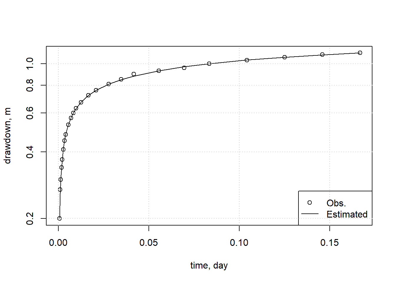
Figure 13.22: Comparison of observed drawdown to those predicted with estimated aquifer characteristics.
The fit is very good in this case, and it should be noted that there are substantial bounds of uncertainty in aquifer parameter estimates.
13.6 Remote sensing of groundwater with GRACE
The Gravity Recovery and Climate Experiment (GRACE) is an international effort (the US lead is NASA) that began collecting data with the launch of a pair of satellites in March 2002. The satellites from GRACE were decomissioned in October 2017, with a follow-on mission (GRACE-FO) launched on May 2018. By making detailed measurements of Earth’s gravitational field, they have been able to estimate changes in water reservoirs over land, ice and oceans.
Data from GRACE are available through each of the research groups involved, with variations in the processing algorithms used to filter, adjust, and correct biases in the measurements. In what follows, data produced by NASA’s Jet Propulsion Lab, distributed by the NASA Earthdata portal. Many variables are distributed with the data, but for groundwater the one of interest is equivalent water thickness (lwe_thickness) expressed in cm. These are referred to as mass concentration blocks, or mascons. After the corrections have been applied, differences in lwe_thickness over time represent an estimate of the change in the mass of water and ice at any location.
The data are distributed by NASA in a single file covering 2002-present for the globe (at a spatial resolution of 0.5 degrees, or about 400 km). For what follows, data distributed with the hydromisc package will be used. What is included below is the preprocessing done to the raw data to reduce the size of the file. Here only the area covering the Western U.S. is included. The preprocessing only uses the terra and geodata packages. These steps may be adapted if more updated data is used or if another region is studied.
# The name of the raw data file from NASA-JPL
grace_file <- "GRCTellus.JPL.200204_202404.GLO.RL06.1M.MSCNv03CRI.nc"

# Only extract lwe_thickness
r <- terra::rast(file.path(grace_file), subds="lwe_thickness")
# download US state boundaries
us_states <- geodata::gadm(country="USA", level=1, path=tempdir())

# Make a new vector layer of only western states
wus_states <- c("Nebraska","Washington","New Mexico","South Dakota","Texas",
                "California","Oregon","Kansas","Idaho","Nevada","Montana",
                "North Dakota","Arizona","Colorado","Oklahoma","Utah","Wyoming")
wus = us_states[match(toupper(wus_states),toupper(us_states$NAME_1)),]

# Project it to ensure it has the same spatial reference as the data
wus_t = terra::project(wus, terra::crs(r))

# Crop out a the desired domain
r_wus <- terra::crop(terra::rotate(r), wus_t, snap="out")

terra::writeCDF(r_wus, "GRCTellus.JPL.200204_202404_wus.nc", varname = "lwe_thickness",
                longname = "Liquid_Water_Equivalent_Thickness",
                unit = "cm")
Example 13.6 Calculate using GRACE satellite data how much water was replenished in the Central Valley between Sept 2014 and Sept 2015 to see if cutbacks resulted in any aquifer recovery. This will replicate some of an early study that used GRACE data to estimate aquifer sustainability. (Famiglietti, 2014). While that reference used (in their Figure 1) September-November averages, we’ll just use Sept values for simplicity.
First, read in the preprocessed file from the hydromisc package.
grace_file <- system.file("extdata", "GRCTellus.JPL.200204_202404_wus.nc", package="hydromisc")
r_wus <- terra::rast(grace_file)
While not shown here, you’ll need the wus_t layer created in the preprocessing step, so run those commands from the preprocessing step. Next, download the shapefile of the aquifer boundary. For California’s central valley, it was obtained from the USGS, which some searching led to here. There are many sources for aquifer boundaries, but in the US starting with the USGS is always productive.
cv_file <- system.file("extdata", "CV_Alluvial_Bnd.shp", package="hydromisc")
cv_bound <- terra::vect(cv_file)

#Convert the spatial reference of the aquifer boundary to match the GRACE data
cv_bound_t = terra::project(cv_bound, terra::crs(r_wus))
The measurement dates are contained in the netcdf file downloaded from NASA, and they are correctly interpreted by terra. Identify the time steps associated with the dates of interest, make sure there is only one measurement for each date (multiple measurements could be averaged, but again for simplicity only one observation is used here). The difference between lwe_thickness between the two dates can then be calculated.
dates <- terra::time(r_wus)
idx1 <- which(dates >= as.Date("2014-09-01") & dates <= as.Date("2014-09-30"))
idx2 <- which(dates >= as.Date("2015-09-01") & dates <= as.Date("2015-09-30"))

# Check to be sure there is exactly one for each
if (length(idx1) != 1 | length(idx2) != 1) message("Must have exactly one index for each date")

# Extract the data for the dates of interest
r1 <- r_wus[[idx1]]
r2 <- r_wus[[idx2]]

# Calculate the liquid water equivalent change over the period
rdelta <- r2 - r1
A preliminary plot can be helpful as a reality check.
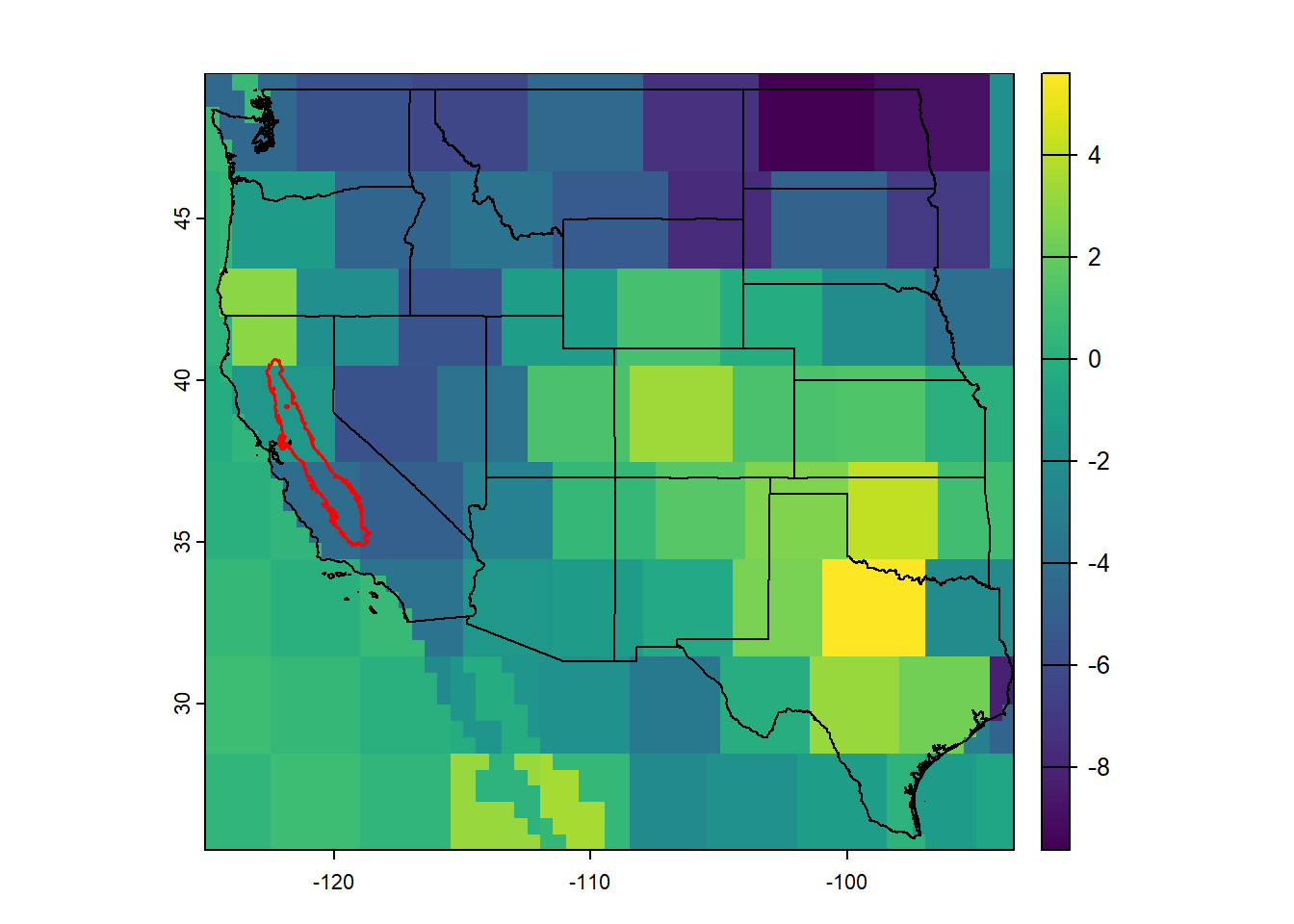
Figure 13.23: Change in water level between Sept 2014 and Sept 2015, cm.
Now crop out only the aquifer extent of interest and plot that.
gw_cv <- terra::crop(rdelta, cv_bound_t, snap="out")
terra::plot(gw_cv)
terra::lines(wus_t)
terra::lines(cv_bound_t, col="red", lwd=1.5)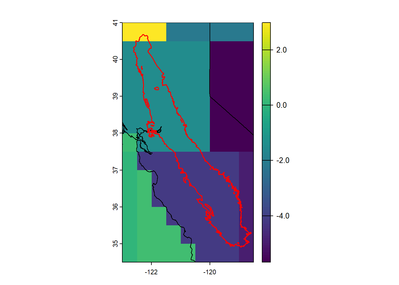
Figure 13.24: Change in water level for the California Central Valley aquifer between Sept 2014 and Sept 2015, cm.
Finally, find the mean change in water storage over this area, and multiply this by the aquifer area to estimate a volume of water.
# Find the area of the CV aquifer
cvaquifer_area <- terra::expanse(cv_bound_t, unit="m")
meanchange <- as.numeric(terra::extract(rdelta, cv_bound_t, fun=mean, ID=FALSE))
cat(sprintf("Aquifer area: %.3e m^2, LWE mean change: %.2f cm\n", cvaquifer_area, meanchange))
#> Aquifer area: 5.324e+10 m^2, LWE mean change: -2.91 cm
volchange <- cvaquifer_area * meanchange/100 # convert to cubic meters
cat(sprintf("Volume change: %.3e m^3\n", volchange))
#> Volume change: -1.547e+09 m^3
Based on this data the aquifer replenishment effort was not successful during this period.