Chapter 10 Designing for floods: flood hydrology
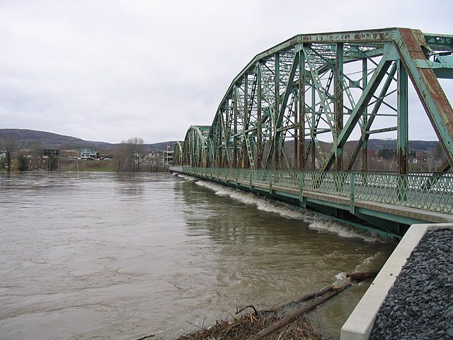
Figure 10.1: The international bridge between Fort Kent, Maine and Clair, New Brunswick during a flood (source: NOAA)
Flood hydrology is generally the description of how frequently a flood of a certain level will be exceeded in a specified period. This was discussed briefly in the section on precipitation frequency, Section 8.3.
The hydromisc package will need to be installed to access some of the data used below. If it is not installed, do so following the instructions on the github site for the package.
10.1 Engineering design requires probability and statistics
Before diving into peak flow analysis, it helps to refresh your background in basic probability and statistics. Some excellent resources for this using R as the primary tool are:
- A very brief tutorial, by Prof. W.B. King
- A more thorough text, by Prof. G. Jay Kerns. This has a companion R package.
- An online flood hydrology reference based in R, by Prof. Helen Fairweather
R functions for distributions use a first letter to designate what it returns: d is the density, p is the (cumulative) probability distribution, q is the quantile, r is a random sequence. For example, a set of 20 normally distributed random numbers can be generated with rnorm(20). Review the King reference above for other examples of using basic statistics in R.
A couple of short demonstrations here will show some of the skills needed for flood hydrology. The first example illustrates binomial probability distribution, which is useful for events with only two possible outcomes (e.g., a flood happens or it doesn’t), where each outcome is independent and probabilities of each are constant. Type ?Binomial in the console to see R documentation on the family of commands for this distribution.
In R the defaults for probabilities are to define them as \(P[X~\le~x]\), or a probability of non-exceedance. Recall that a probability of exceedance is simply 1 - (probability of non-exceedance), or \(P[X~\gt~x] ~=~ 1-P[X~\le~x]\). In R, for quantiles or probabilities (using functions beginning with q or p like pnorm or qlnorm) setting the argument lower.tail to FALSE uses a probability of exceedance instead of non-exceedance.
Example 10.1 A temporary dam is constructed while a repair is built. It will be in place 5 years and is designed to protect against floods up to a 20-year recurrence interval (i.e., there is a \(p=\frac{1}{20}=0.05\), or 5% chance, that it will be exceeded in any one year). What is the probability of (a) no failure in the 5 year period, and (b) at least two failures in 5 years.
# (a)
ans1 <- dbinom(0, 5, 0.05)
cat(sprintf("Probability of exactly zero occurrences in 5 years = %.4f %%",100*ans1))
#> Probability of exactly zero occurrences in 5 years = 77.3781 %
# (b)
ans2 <- 1 - pbinom(1,5,.05) # or pbinom(1,5,.05, lower.tail=FALSE)
cat(sprintf("Probability of 2 or more failures in 5 years = %.2f %%",100*ans2))
#> Probability of 2 or more failures in 5 years = 2.26 %
While the next example uses normally distributed data, most data in hydrology are better described by other distributions.
Example 10.2 Annual average streamflows in some location are normally distributed with a mean annual flow of 20 m\(^3\)/s and a standard deviation of 6 m\(^3\)/s. Find (a) the probability of experiencing a year with less than (or equal to) 10 m\(^3\)/s, (b) greater than 32 m\(^3\)/s, and (c) the annual average flow that would be expected to be exceeded 10% of the time.
# (a)
ans1 <- pnorm(10, mean=20, sd=6)
cat(sprintf("Probability of less than 10 = %.2f %%",100*ans1))
#> Probability of less than 10 = 4.78 %
# (b)
ans2 <- pnorm(32, mean=20, sd=6, lower.tail = FALSE) #or 1 - pnorm(32, mean=20, sd=6)
cat(sprintf("Probability of greater than or equal to 30 = %.2f %%",100*ans2))
#> Probability of greater than or equal to 30 = 2.28 %
# (c)
ans3 <- qnorm(.1, mean=20, sd=6, lower.tail=FALSE)
cat(sprintf("flow exceeded 10%% of the time = %.2f m^3/s",ans3))
#> flow exceeded 10% of the time = 27.69 m^3/s
# plot to visualize answers
x <- seq(0,40,0.1)
y<- pnorm(x,mean=20,sd=6)
xlbl <- expression(paste(Flow, ",", ~ m^"3"/s))
plot(x ,y ,type="l",lwd=2, xlab = xlbl, ylab= "Prob. of non-exceedance")
abline(v=10,col="black", lwd=2, lty=2)
abline(v=32,col="blue", lwd=2, lty=2)
abline(h=0.9,col="green", lwd=2, lty=2)
legend("bottomright",legend=c("(a)","(b)","(c)"),col=c("black","blue","green"), cex=0.8, lty=2)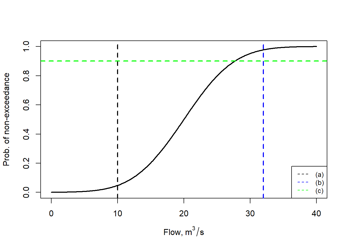
Figure 10.2: Illustration of three solutions.
10.2 Estimating floods when you have peak flow observations - flood frequency analysis
For an area fortunate enough to have a long record (several decades or more) of observations, estimating flood risk is a matter of statistical data analysis. In the U.S., data, collected by the U.S. Geological Survey (USGS), can be accessed through the National Water Dashboard. Sometimes for discontinued stations it is easier to locate data through the older USGS map interface. For any site, data may be downloaded to a file, and the peakfq (watstore) format, designed to be imported into the PeakFQ software. As of late 2024, there is a USGS web app that retrieves peak flow data for any gauge, obviating the need to download data separately.It is easy to work with USGS flow data, including instantaneous peak flows, in R, since data can also be accessed directly.
10.2.1 Installing helpful packages
The USGS has developed many R packages, including one for retrieval of data, dataRetrieval. Since this resides on CRAN, the package can be installed with (the use of ‘!requireNamespace’ skips the installation if it already is installed):
Other USGS packages that are very helpful for peak flow analysis are not on CRAN, but rather housed in a USGS repository. The easiest way to install packages from that archive is to follow the installation instructions at that repository. For the exercises below, install smwrGraphs and smwrBase following the instructions at those sites. The prefix smwr refers to their use in support of the excellent reference Statistical Methods in Water Resources.
Lastly, the lmomco package has extensive capabilities to work with many forms of probability distributions, and has functions for calculating distribution parameters (like skew) that we will use.
10.2.2 Download, manipulate, and plot the data for a site
Using the older USGS site mapper, and specifying that inactive stations should also be included, many stations in the south Bay Area in California are shown in Figure 10.3.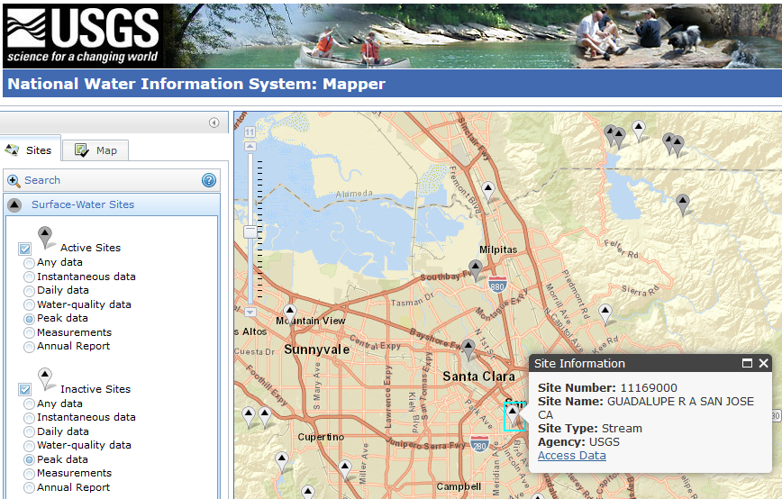
Figure 10.3: Active and Inactive USGS sites recording peak flows.
While the data could be downloaded and saved locally through that link, it is convenient here to use the dataRetrieval command. Note that this package is being rewritten, and commands are changing as revisions occur.
The data used here are also available as part of the hydromisc package, and may be obtained by typing hydromisc::Qpeak_download.
It is always helpful to look at the downloaded data frame before doing anything with it. There are many columns that are not needed or that have repeated information. There are also some rows that have no data (‘NA’ values). It is also useful to change some column names to something more intuitive. We will need to define the water year (a water year begins October 1 and ends September 30).
Qpeak <- Qpeak_download[!is.na(Qpeak_download$peak_dt),c('peak_dt','peak_va')]
colnames(Qpeak)[colnames(Qpeak)=="peak_dt"] <- "Date"
colnames(Qpeak)[colnames(Qpeak)=="peak_va"] <- "Peak"
Qpeak$wy <- smwrBase::waterYear(Qpeak$Date)
The data have now been simplified so that can be used more easily in the subsequent flood frequency analysis. Data should always be plotted, which can be done many ways. As a demonstration of highlighting specific years in a barplot, the strongest El Niño years (in 1930-2002) from NOAA Physical Sciences Lab can be highlighted in red.
xlbl <- "Water Year"
ylbl <- expression("Peak Flow, " ~ ft^{3}/s)
nino_years <- c(1983,1998,1992,1931,1973,1987,1941,1958,1966, 1995)
cols <- c("blue", "red")[(Qpeak$wy %in% nino_years) + 1]
barplot(Qpeak$Peak, names.arg = Qpeak$wy, xlab = xlbl, ylab=ylbl, col=cols)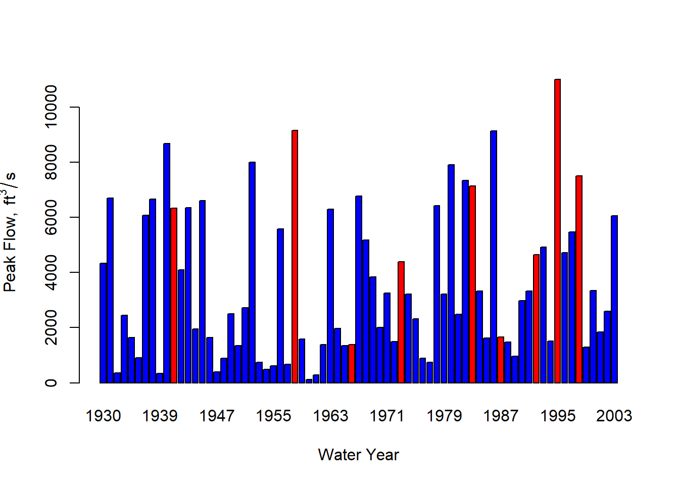
Figure 10.4: Annual peak flows for USGS gauge 11169000, highlighting strong El Niño years in red.
10.2.3 Flood frequency analysis
The general formula used for flood frequency analysis is Equation (10.1). \[\begin{equation} y=\overline{y}+Ks_y \tag{10.1} \end{equation}\] where y is the flow at the designated return period, \(\overline{y}\) is the mean of all \(y\) values and \(s_y\) is the standard deviation. In most instances, \(y\) is a log-transformed flow; in the US a base-10 logarithm is generally used. \(K\) is a frequency factor, which is a function of the return period, the parent distribution, and often the skew of the y values. The guidance of the USGS (as in Guidelines for Determining Flood Flow Frequency, Bulletin 17C) (England, J.F. et al., 2019) is to use the log-Pearson Type III (LP-III) distribution for flood frequency data, though in different settings other distributions can perform comparably. For using the LP-III distribution, we will need several statistical properties of the data: mean, standard deviation, and skew, all of the log-transformed data, calculated as follows.
mn <- mean(log10(Qpeak$Peak))
std <- sd(log10(Qpeak$Peak))
g <- lmomco::pmoms(log10(Qpeak$Peak))$skew
With those calculated, a defined return period can be chosen and the flood frequency factors, from Equation (10.1), calculated for that return period (the example here is for a 50-year return period). The qnorm function from base R and the qpearsonIII function from the smwrBase package make this straightforward, and K values for Equation (10.1) are obtained for a lognormal, Knorm, and LP-III, Klp3.
Now the flood frequency equation (10.1) can be applied to calculate the flows associated with the 50-year return period for each of the distributions. Remember to take the anti-log of your answer to return to standard units.
10.2.4 Creating a flood frequency plot
Different probability distributions can produce very different results for a design flood flow. Plotting the historical observations along with the distributions, the lognormal and LP-III in this case, can help explain why they differ, and provide indications of which fits the data better.
We cannot say exactly what the probability of seeing any observed flood exceeded would be. However, given a long record, the probability can be described using the general “plotting position” equation from Bulletin 17C, as in Equation (10.2). \[\begin{equation} p_i=\frac{i-a}{n+1-2a} \tag{10.2} \end{equation}\] where n is the total number of data points (annual peak flows in this case), \(p_i\) is the exceedance probability of flood observation i, where flows are ranked in descending order (so the largest observed flood has \(i=1\) ad the smallest is \(i=n\)). The parameter a is between 0 and 0.5. For simplicity, the following will use \(a=0\), so the plotting Equation (10.2) becomes the Weibull formula, Equation (10.3). \[\begin{equation} p_i=\frac{i}{n+1} \tag{10.3} \end{equation}\]
While not necessary, to add probabilities to the annual flow sequence we will create a new data frame consisting of the observed peak flows, sorted in descending order.
This can be done with fewer commands, but here is an example where first a rank column is created (1=highest peak in the record of N years), followed by adding columns for the exceedance and non-exceedence probabilities:
df_pp$rank <- as.integer(seq(1:length(df_pp$Obs_peak)))
df_pp$exc_prob <- (df_pp$rank/(1+length(df_pp$Obs_peak)))
df_pp$ne_prob <- 1-df_pp$exc_prob
For each of the non-exceedance probabilities calculated for the observed peak flows, use the flood frequency equation (10.1) to estimate the peak flow that would be predicted by a lognormal or LP-III distribution. This is the same thing that was done above for a specified return period, but now it will be “applied” to an entire column.
df_pp$LN_peak <- mapply(function(x) {10^(mn+std*qnorm(x))}, df_pp$ne_prob)
df_pp$LP3_peak <- mapply(function(x) {10^(mn+std*smwrBase::qpearsonIII(x, skew=g))},df_pp$ne_prob)
There are many packages that create probability plots (see, for example, the versatile scales package for ggplot2). For this example the USGS smwrGraphs package is used. First, for aesthetics, create x- and y- axis labels.
The smwrGraphs package works most easily if it writes output directly to a file, a PNG file in this case, using the setPNG command; the file name and its dimensions in inches are given as arguments, and the PNG device is opened for writing. This is followed by commands to plot the data on a graph. Technically, the data are plotted to an object here is called prob.pl. The probPlot command plots the observed peaks as points, where the alpha argument is the a in Equation (10.2). Additional points or lines are added with the addXY command, used here to add the LN and LP3 data as lines (one solid, one dashed). Finally, a legend is added (the USGS refers to that as an “Explanation”), and the output PNG file is closed with the dev.off() command.
smwrGraphs::setPNG("probplot_smwr.png",6.5, 3.5)
#>  width height
#>    6.5    3.5
#> [1] "Setting up markdown graphics device:  probplot_smwr.png"
prob.pl <- smwrGraphs::probPlot(df_pp$Obs_peak, alpha = 0.0, Plot=list(what="points",size=0.05,name="Obs"), xtitle=xlbl, ytitle=ylbl)
prob.pl <- smwrGraphs::addXY(df_pp$ne_prob,df_pp$LN_peak,Plot=list(what="lines",name="LN"),current=prob.pl)
prob.pl <- smwrGraphs::addXY(df_pp$ne_prob,df_pp$LP3_peak,Plot=list(what="lines",type="dashed",name="LP3"),current=prob.pl)
smwrGraphs::addExplanation(prob.pl,"ul",title="")
dev.off()
#> png
#>   2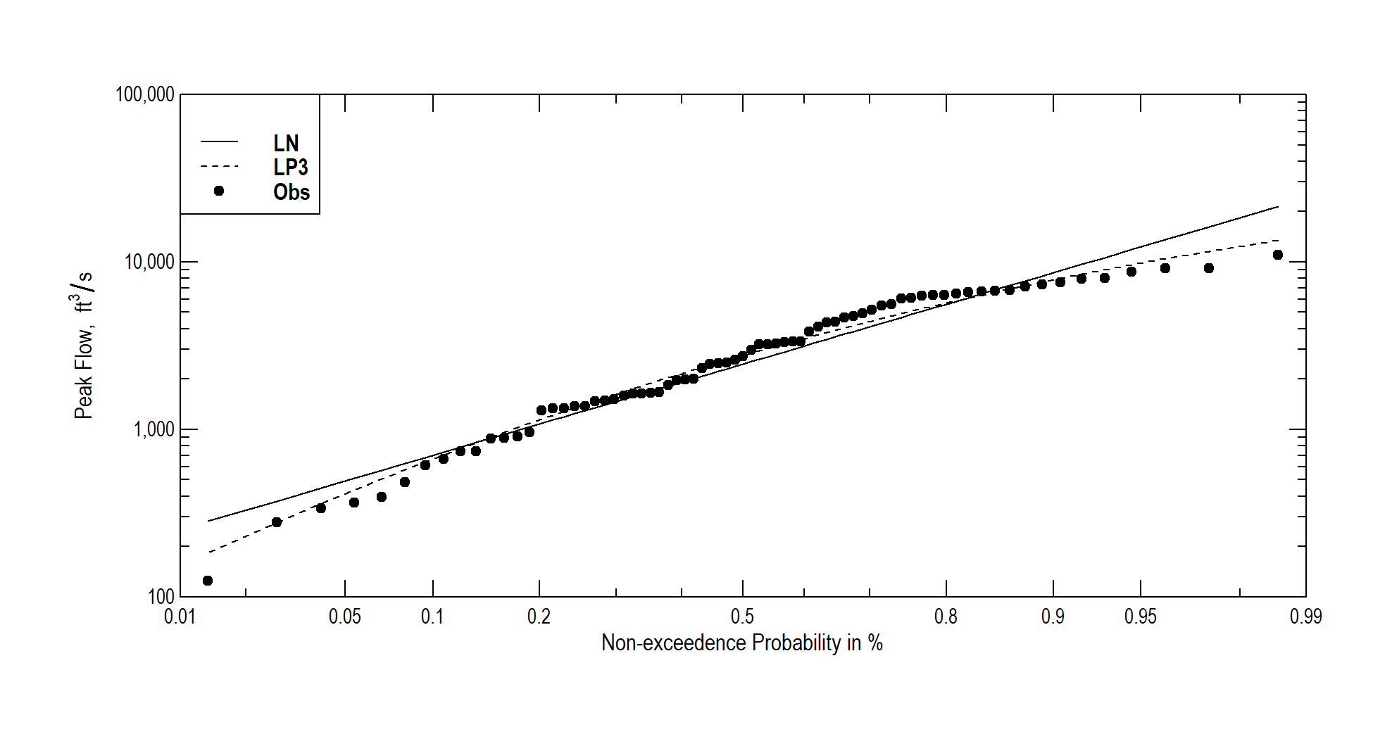
Figure 10.5: Probability plot for USGS gauge 11169000 for years 1930-2002.
10.2.5 Other software for peak flow analysis
Much of the analysis above can be achieved using the PeakFQ software developed by the USGS. It incorporates the methods in Bulletin 17C via a graphical interface and can import data in the watstore format as discussed above in Section 10.2.
The USGS has also produced the MGBT R package to perform many of the statistical calculations involved in the Bulletin 17C procedures.
10.3 Estimating floods from precipitation
When extensive streamflow data are not available, flood risk can be estimated from precipitation and the characteristics of the area contributing flow to a point. While not covered here (or not yet…), there has been extensive development of hydrological modeling using R, summarized in recent papers (Astagneau et al., 2021; Slater et al., 2019).
Straightforward application of methods to estimate peak flows or hydrographs resulting from design storms can by writing code to apply the Rational Formula (included in the VFS and hydRopUrban packages, for example) or the NRCS peak flow method.
For more sophisticated analysis of water supply and drought, continuous modeling is required. A very good introduction to hydrological modeling in R, including model calibration and assessment, is included in the Hydroinformatics at VT reference by JP Gannon.