Chapter 5 Flow in open channels
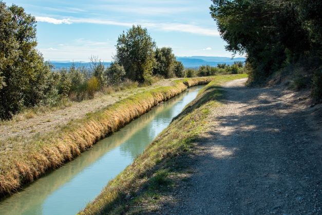
Where flowing water water is exposed to the atmosphere, and thus not under pressure, its condition is called open channel flow.
Typical design challenges can be:
- Determining how deep water will flow in a channel
- Finding the bottom slope required to carry a defined flow in a channel
- Comparing different cross-sectional shapes and dimensions to carry flow
In pipe flow the cross-sectional area does not change with flow rate, which simplifies some aspects of calculations. By contrast, in open channel flow conditions including flow depth, area, and roughness can all vary with flow rate, which tends to make the equations more cumbersome. In civil engineering applications, roughness characteristics are not usually considered as variable with flow rate.
In what follows, three conditions for flow are considered:
- Uniform flow, where flow characteristics do not vary along the length of a channel
- Gradually varied flow, where flow responds to an obstruction or change in channel conditions with a gradual adjustment in flow depth
- Rapidly varied flow, where an abrupt channel transition results in a rapid change in water surface, the most important case of which is the hydraulic jump
5.1 An important dimensionless quantity
For open channel flow, given a channel shape and flow rate, flow can usually exist at two different depths, termed subcritical (slow, deep) and supercritical (shallow, fast). The exception is at critical flow conditions, where only one depth exists, the critical depth. Which of these depths is exhibited by the flow is determined by the slope and roughness of the channel.
The Froude number characterizes whether flow is critical, supercritical or subcritical, and is defined by Equation (5.1)
\[\begin{equation} Fr=\frac{V}{\sqrt{gD}} \tag{5.1} \end{equation}\]
The Froude number characterizes flow as:
| Fr | Condition | Description |
|---|---|---|
| <1.0 | subcritical | slow, deep |
| =1.0 | critical | undulating, transitional |
| >1.0 | supercritical | fast, shallow |
Critical flow is important in open-channel flow applications and is discussed further below.
5.2 Equations for open channel flow
Flow conditions in an open channel under uniform flow conditions are often related by the Manning equation (5.2). \[\begin{equation} Q=A\frac{C}{n}{R}^{\frac{2}{3}}{S}^{\frac{1}{2}} \tag{5.2} \end{equation}\]
In Equation (5.2), C is 1.0 for SI units and 1.49 for Eng (British Gravitational, English., or U.S. Customary) units. Q is the flow rate, A is the cross-sectional flow area, n is the Manning roughness coefficient, S is the longitudinal channel slope, and R is the hydraulic radius, defined by equation (5.3) \[\begin{equation} R=\frac{A}{P} \tag{5.3} \end{equation}\] where P is the wetted perimeter.
Critical depth is defined by the relation (at critical conditions) in Equation (5.4) \[\begin{equation} \frac{Q^{2}B}{g\,A^{3}}=1 \tag{5.4} \end{equation}\] where B is the width of the water surface (top width).
Because of the channel geometry being included in A and R, it helps to work with specific shapes in adapting these equations. The two most common are trapezoidal and circular, included in Sections 5.3 and 5.4 below.
As with pipe flow, the energy equation applies for one dimensional open channel flow as well, Equation (5.5): \[\begin{equation} \frac{V_1^2}{2g}+y_1+z_1=\frac{V_2^2}{2g}+y_2+z_2+h_L \tag{5.5} \end{equation}\] where point 1 is upstream of point 2, V is the flow velocity, y is the flow depth, and z is the elevation of the channel bottom. \(h_L\) is the energy head loss from point 1 to point 2. For uniform flow, \(h_L\) is the drop in elevation between the two points due to the channel slope.
5.3 Trapezoidal channels
In engineering applications one of the most common channel shapes is trapezoidal.
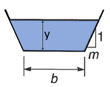
Figure 5.1: Typical symmetrical trapezoidal cross section
The geometrical relationships for a trapezoid are: \[\begin{equation} A=(b+my)y \tag{5.6} \end{equation}\]
\[\begin{equation} P=b+2y\sqrt{1+m^2} \tag{5.7} \end{equation}\]
Combining Equations (5.6) and (5.7) yields: \[\begin{equation} R=\frac{A}{P}=\frac{\left(b+my\right)y}{b+2y\sqrt{1+m^2}} \tag{5.8} \end{equation}\]
Top width: \(B=b+2\,m\,y\).
Substituting Equations (5.6) and (5.8) into the Manning equation produces Equation (5.9). \[\begin{equation} Q=\frac{C}{n}{\frac{\left(by+my^2\right)^{\frac{5}{3}}}{\left(b+2y\sqrt{1+m^2}\right)^\frac{2}{3}}}{S}^{\frac{1}{2}} \tag{5.9} \end{equation}\]
5.3.1 Solving the Manning equation in R
To solve Equation (5.9) when any variable other than Q is unknown, it is straightforward to rearrange it to a form of y(x) = 0. \[\begin{equation} Q-\frac{C}{n}{\frac{\left(by+my^2\right)^{\frac{5}{3}}}{\left(b+2y\sqrt{1+m^2}\right)^\frac{2}{3}}}{S}^{\frac{1}{2}}=0 \tag{5.10} \end{equation}\] This allows the use of a standard solver to find the root(s). If solving it by hand, trial and error can be employed as well.
Example 5.1 demonstrates the solution of Equation (5.10) for the flow depth, y. A trial-and-error approach can be applied, and with careful selection of guesses a solution can be obtained relatively quickly. Using solvers makes the process much quicker and less prone to error.
Example 5.1 Find the flow depth, y, for a trapezoidal channel with Q=225 ft3/s, n=0.016, m=2, b=10 ft, S=0.0006.
The Manning equation can be set up as a function in terms of a missing variable, here using normal depth, y as the missing variable.
yfun <- function(y) {
  Q - (((y * (b + m * y)) ^ (5 / 3) * sqrt(S)) * (C / n) / ((b + 2 * y * sqrt(1 + m ^ 2)) ^ (2 / 3)))
  }
Because these use US Customary (or English) units, C=1.486. Define all of the needed input variables for the function.
Use the R function uniroot to find a single root within a defined interval. Set the interval (the range of possible y values in which to search for a root) to cover all plausible values, here from 0.0001 mm to 200 m.
ans <- uniroot(yfun, interval = c(0.0000001, 200), extendInt = "yes")
cat(sprintf("Normal Depth: %.3f ft\n", ans$root))
#> Normal Depth: 3.406 ft
Functions can usually be given multiple values as input, returning the corresponding values of output. this allows plots to be created to show, for example, how the left side of Equation (5.10) varies with different values of depth, y.
ys <- seq(0.1, 5, 0.1)
plot(ys,yfun(ys), type='l', xlab = "y, ft", ylab = "Function to solve for zero")
abline(h=0)
grid()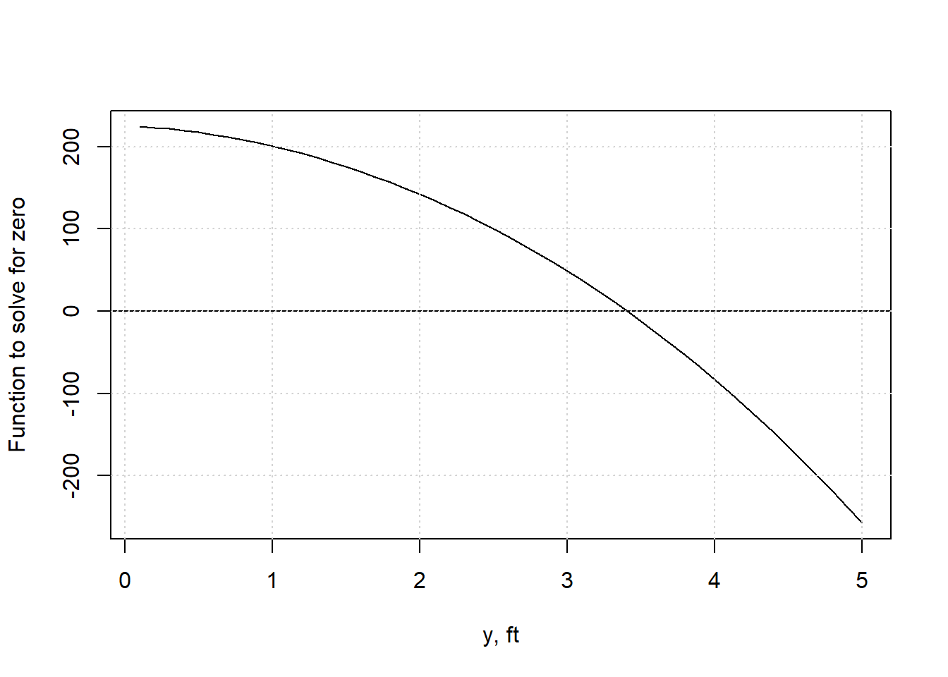
This validates the result in the example, showing the root of Equation (5.10), when the function has a value of 0, occurs for a depth, y of a little less than 3.5.
5.3.2 Solving the Manning equation with the hydraulics R package
The hydraulics package has a manningt (the ‘t’ is for ‘trapezoid’) function for trapezoidal channels. Example 5.2 demonstrates its usage.
Example 5.2 Find the uniform (normal) flow depth, y, for a trapezoidal channel with Q=225 ft3/s, n=0.016, m=2, b=10 ft, S=0.0006.
Specifying “Eng” units ensures the correct C value is used. Sf is the same as S in Equations (5.2) and (5.9) since flow is uniform.
ans <- hydraulics::manningt(Q = 225., n = 0.016, m = 2, b = 10., Sf = 0.0006, units = "Eng")
cat(sprintf("Normal Depth: %.3f ft\n", ans$y))
#> Normal Depth: 3.406 ft
#critical depth is also returned, along with other variables.
cat(sprintf("Critical Depth: %.3f ft\n", ans$yc))
#> Critical Depth: 2.154 ft
5.3.3 Solving the Manning equation using a spreadsheet like Excel
Spreadsheet software is very popular and has been modified to be able to accomplish many technical tasks such as solving equations. This example uses Excel with its solver add-in activated, though other spreadsheet software has similar solver add-ins that can be used.
The first step is to enter the input data, for the same example as above, along with an initial guess for the variable you wish to solve for. The equation for which a root will be determined is typed in using the initial guess for y in this case.
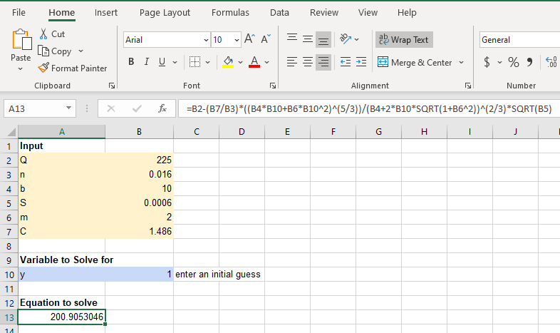
At this point you could use a trial-and-error approach and simply try different values for y until the equation produces something close to 0.
A more efficient method is to use a solver. Check that the solver add-in is activated (in Options) and open it. Set the values appropriately.
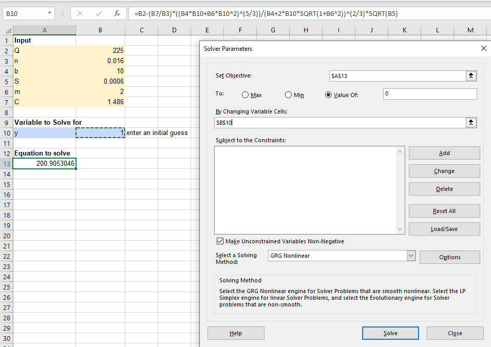
Click Solve and the y value that produces a zero for the equation will appear.
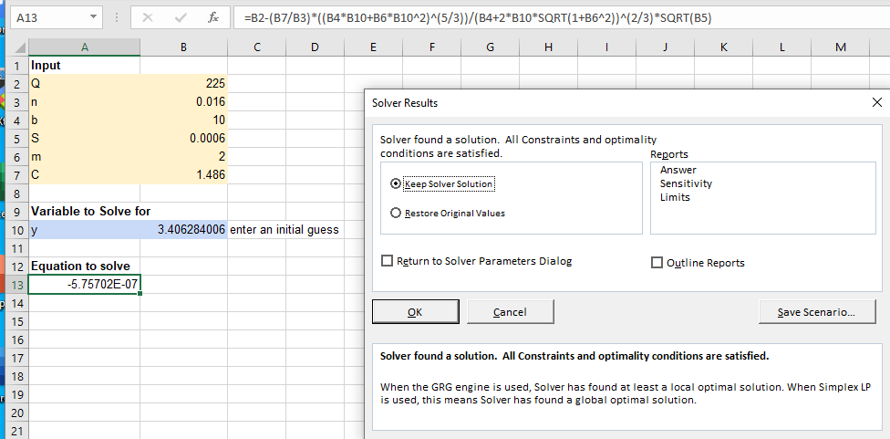
If you need to solve for multiple roots, you will need to start from different initial guesses.
5.3.4 Optimal trapezoidal geometry
Most fluid mechanics texts that include open channel flow include a derivation of optimal geometry for a trapezoidal channel. This is also called the most efficient cross section. What this means is for a given A and m, there is an optimal flow depth and bottom width for the channel, defined by Equations (5.11) and (5.12).
\[\begin{equation} b_{opt}=2y\left(\sqrt{1+m^2}-m\right) \tag{5.11} \end{equation}\] \[\begin{equation} y_{opt}=\sqrt{\frac{A}{2\sqrt{1+m^2}-m}} \tag{5.12} \end{equation}\]
These may be calculated manually, but they are also returned by the manningt function of the hydraulics package in R. Example 5.3 demonstrates this.
Example 5.3 Find the optimal channel width to transmit 360 ft3/s at a depth of 3 ft with n=0.015, m=1, S=0.0006.
ans <- hydraulics::manningt(Q = 360., n = 0.015, m = 1, y = 3.0, Sf = 0.00088, units = "Eng")
knitr::kable(format(as.data.frame(ans), digits = 2), format = "pipe", padding=0)| Q | V | A | P | R | y | b | m | Sf | B | n | yc | Fr | Re | bopt |
|---|---|---|---|---|---|---|---|---|---|---|---|---|---|---|
| 360 | 5.3 | 68 | 28 | 2.4 | 3 | 20 | 1 | 0.00088 | 26 | 0.015 | 2.1 | 0.57 | 1159705 | 4.8 |
The results show that, aside from the rounding, the required width is approximately 20 ft, and the optimal bottom width for optimal hydraulic efficiency would be 4.76 ft. To check the depth that would be associated with a channel of the optimal width, substitute the optimal width for b and solve for y:
5.4 Circular Channels (flowing partially full)
Civil engineers encounter many situations with circular pipes that are flowing only partially full, such as storm and sanitary sewers.
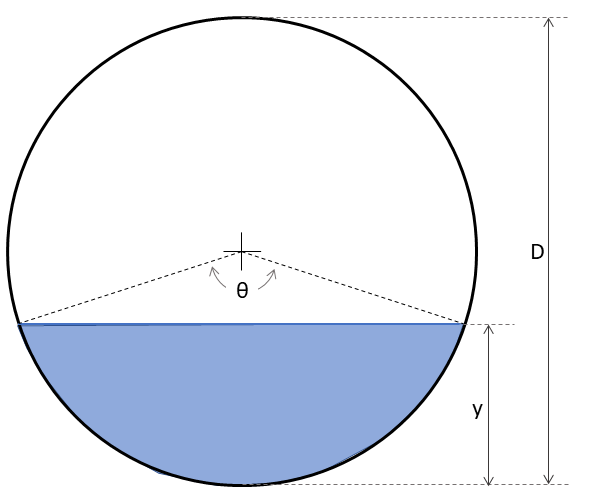
Figure 5.3: Typical circular cross section
The relationships between the depth of water and the values needed in the Manning equation are:
Depth (or fractional depth as written here) is described by Equation (5.13) \[\begin{equation} \frac{y}{D}=\frac{1}{2}\left(1-\cos{\frac{\theta}{2}}\right) \tag{5.13} \end{equation}\]
Area is described by Equation (5.14) \[\begin{equation} A=\left(\frac{\theta-\sin{\theta}}{8}\right)D^2 \tag{5.14} \end{equation}\] (Be sure to use theta in radians.)
Wetted perimeter is described by Equation (5.15) \[\begin{equation} P=\frac{D\theta}{2} \tag{5.15} \end{equation}\]
Combining Equations (5.14) and (5.15): \[\begin{equation} R=\frac{D}{4}\left(1-\frac{\sin{\theta}}{\theta}\right) \tag{5.16} \end{equation}\]
Top width: \(B=D\,sin{\frac{\theta}{2}}\)
Substituting Equations (5.14) and (5.16) into the Manning equation, Equation (5.2), produces (5.17). \[\begin{equation} \theta^{-\frac{2}{3}}\left(\theta-\sin{\theta}\right)^\frac{5}{3}-CnQD^{-\frac{8}{3}}S^{-\frac{1}{2}}=0 \tag{5.17} \end{equation}\] where C=20.16 for SI units and C=13.53 for US Customary (English) units.
5.4.1 Solving the Manning equation for a circular pipe in R
As was demonstrated with pipe flow, a function could be written with Equation (5.17) and a solver applied to find the value of \(\theta\) for the given flow conditions with a known D, S, n and Q. The value for \(\theta\) could then be used with Equations (5.13), (5.14) and (5.15) to recover geometric values.
Hydraulic analysis of circular pipes flowing partially full often account for the value of Manning’s n varying with depth (Camp, 1946); some standards recommend fixed n values, and others require the use of a depth-varying n. The R package hydraulics has implemented those routines to enable these calculations, including using a fixed n (the default) or a depth-varing n.
For an existing pipe, a common problem is the determination of the depth, y that a given flow Q, will have given a pipe diameter d, slope S and roughness n. Example 5.4 demonstrates this.
Example 5.4 Find the uniform (normal) flow depth, y, for a trapezoidal channel with Q=225 ft3/s, n=0.016, m=2, b=10 ft, S=0.0006. Do this assuming both that Manning n is constant with depth and that it varies with depth.
The function manningc from the hydraulics package is used. Any one of the variables in the Manning equation, and related geometric variables, may be treated as an unknown.
ans <- hydraulics::manningc(Q=0.01, n=0.013, Sf=0.001, d = 0.2, units="SI", ret_units = TRUE)
ans2 <- hydraulics::manningc(Q=0.01, n=0.013, Sf=0.001, d = 0.2, n_var = TRUE, units="SI", ret_units = TRUE)
df <- data.frame(Constant_n = unlist(ans), Variable_n = unlist(ans2))
knitr::kable(df, format = "html", digits=3, padding = 0, col.names = c("Constant n","Variable n")) |>
kableExtra::kable_styling(full_width = F)| Constant n | Variable n | |
|---|---|---|
| Q | 0.010 | 0.010 |
| V | 0.376 | 0.344 |
| A | 0.027 | 0.029 |
| P | 0.437 | 0.482 |
| R | 0.061 | 0.060 |
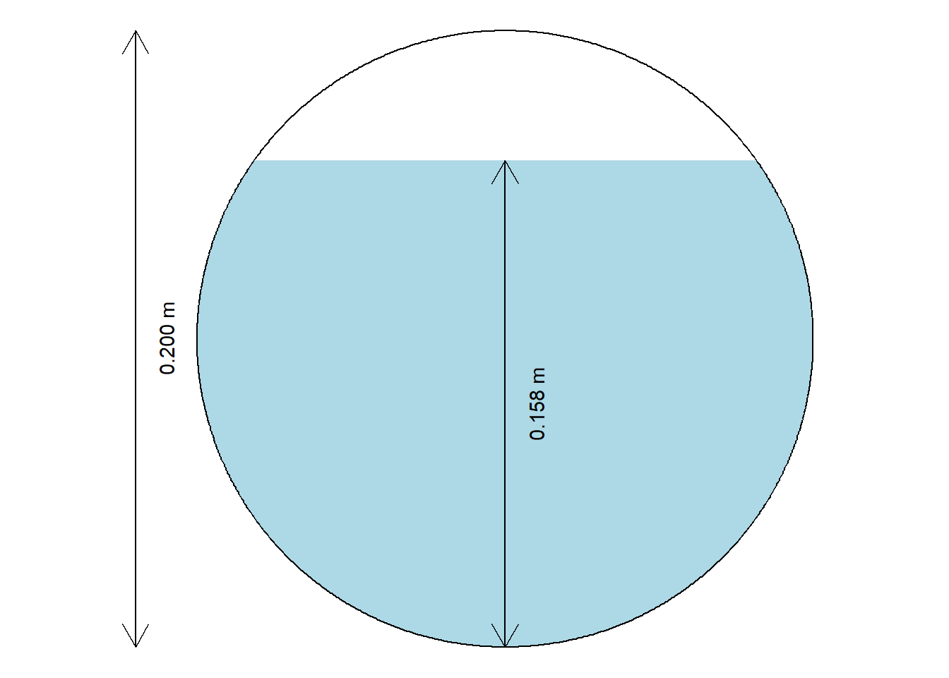
| y | 0.158 | 0.174 |
| d | 0.200 | 0.200 |
| Sf | 0.001 | 0.001 |
| n | 0.013 | 0.014 |
| yc | 0.085 | 0.085 |
| Fr | 0.297 | 0.235 |
| Re | 22342.979 | 20270.210 |
| Qf | 0.010 | 0.010 |
It is also sometimes convenient to see a cross-section diagram.
5.5 Critical flow
Critical flow in open channel flow is described in general by Equation (5.4).
For any channel geometry and flow rate a convenient plot is a specific energy diagram, which illustrates the different flow depths that can occur for any given specific energy. Specific energy is defined by Equation (5.18). \[\begin{equation} E=y+\frac{V^2}{2g} \tag{5.18} \end{equation}\] It can be interpreted as the total energy head, or energy per unit weight, relative to the channel bottom.
For a trapezoidal channel, critical flow conditions occur as described by Equation (5.4). Combining that with trapezoidal geometry produces Equation (5.19) \[\begin{equation} \frac{Q^2}{g}=\frac{\left(by_c+m{y_c}^2\right)^3}{b+2my_c} \tag{5.19} \end{equation}\] where \(y_c\) indicates critical flow depth.
This is important for understanding what may happen to the water surface when flow encounters an obstacle or transition. For the channel of Example 5.3, the diagram is shown in Figure 5.4.
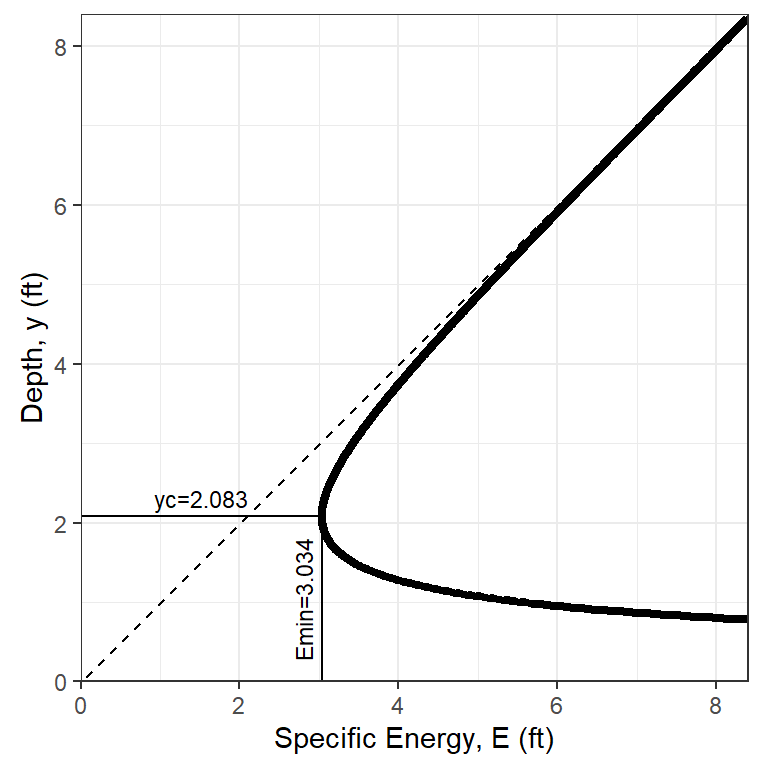
Figure 5.4: A specific energy diagram for the conditions of Example 5.3.
This provides an illustration that for y=3 ft the flow is subcritical (above the critical depth). Specific energy for the conditions of the prior example is \[E=y+\frac{V^2}{2g}=3.0+\frac{5.22^2}{2*32.2}=3.42 ft\]
If the channel bottom had an abrupt rise of \(E-E_c=3.42-3.03=0.39 ft\) critical depth would occur over the hump. A rise of anything greater than that would cause damming to occur. Once flow over a hump is critical, downstream of the hump the flow will be in supercritical conditions, flowing at the alternate depth.
The specific energy for a given depth y and alternate depth can be added to the plot by including an argument for depth, y, as in Figure 5.5.
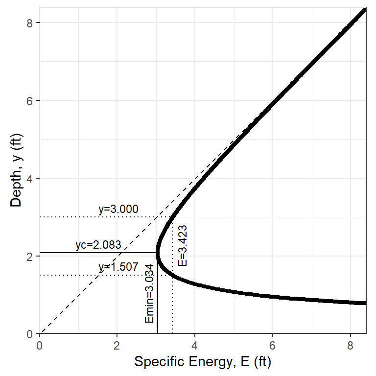
Figure 5.5: A specific energy diagram for the conditions of Example 5.3 with an additional y value added.
5.6 Flow in Rectangular Channels
When working with rectangular channels the open channel equations simplify, because flow, \(Q\), can be expressed as flow per unit width, \(q = Q/b\), where \(b\) is the channel width. Since \(Q/A=V\) and \(A=by\), Equation (5.18) can be written as Equation (5.20):
\[\begin{equation} E=y+\frac{Q^2}{2gA^2}=y+\frac{q^2}{2gy^2} \tag{5.20} \end{equation}\]
Equation (5.19) for critical depth, \(y_c\), also is simplified for rectangular channels to Equation (5.21):
\[\begin{equation} y_c = \left({\frac{q^2}{g}}\right)^{1/3} \tag{5.21} \end{equation}\]
Combining Equation (5.20) and Equation (5.21) shows that at critical conditions, the minimum specific energy is:
\[\begin{equation} E_{min} = \frac{3}{2} y_c \tag{5.22} \end{equation}\]
Example 5.5, based on an exercise from the open-channel flow text by Sturm (Sturm, 2021), demonstrates how to solve for the depth through a rectangular section when the bottom height changes.
Example 5.5 A 0.5 m wide rectangular channel carries a flow of 2.2 m\(^3\)/s at a depth of 2 m (\(y_1\)=2m). If the channel bottom rises 0.25 m (\(\Delta z=0.25~ m\)), and head loss, \(h_L\) over the transition is negligible, what is the depth, \(y_2\) after the rise in channel bottom?
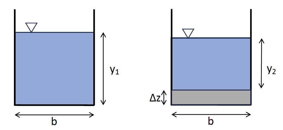
Figure 5.6: The rectangular channel of Example 5.5 with an increase in channel bottom height downstream.
A specific energy diagram is very helpful for establishing upstream conditions and estimating \(y_2\).
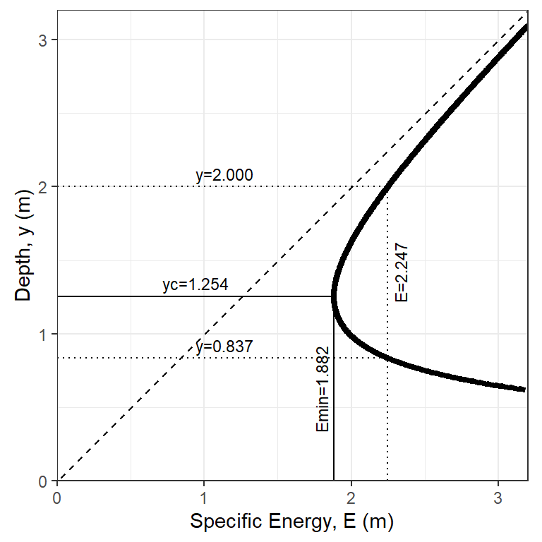
Figure 5.7: A specific energy diagram for the conditions of Example 5.5.
The values of \(y_c\) and \(E_{min}\) shown in the plot can be verified using Equations (5.21) and (5.22). This should always be checked to describe the incoming flow and what will happen as flow passes over a hump. Since \(y_1\) > \(y_c\) the upstream flow is subcritical, and flow can be expected to drop as it passes over the hump. Upstream and downstream specific energy are related by Equation (5.23):
\[\begin{equation} E_1-E_2=\Delta z + h_L \tag{5.23} \end{equation}\] Since \(h_L\) is negligible in this example, the downstream specific energy, \(E_2\) is lower that the upper \(E_1\) by an amount \(\Delta z\), or \[\begin{equation} E_2 = E_1 - \Delta z \tag{5.24} \end{equation}\]
For a 0.25 m rise, and using \(q = Q/b = 2.2/0.5 = 4.4\), combining Equation (5.24) and Equation (5.20):
\[E_2 = E_1 - 0.25 = 2 + \frac{4.4^2}{2(9.81)(2^2)} - 0.25 = 2.247 - 0.25 = 1.997 ~m\]
From the specific energy diagram, for \(E_2=1.997 ~ m\) a depth of about \(y_2 \approx 1.6 ~ m\) would be expected, and the flow would continue in subcritical conditions. The value of \(y_2\) can be calculated using Equation (5.20):
\[1.997 = y_2 + \frac{4.4^2}{2(9.81)(y_2^2)}\] which can be rearranged to \[0.9967 - 1.997 y_2^2 + y_2^3= 0\]
Solving a polynomial in R is straightforward using the polyroot function and using Re to extract the real portion of the solution (after filtering for non-imaginary solutions).
all_roots <- polyroot(c(0.9667, 0, -1.997, 1))
Re(all_roots)[abs(Im(all_roots)) < 1e-6]
#> [1]  0.9703764 -0.6090519  1.6356755
The negative root is meaningless, the lower positive root is the supercritical depth for \(E_2 = 1.997 ~ m\), and the larger positive root is the subcritical depth. Thus the correct solution is \(y_2 = 1.64 ~ m\) when the channel bottom rises by 0.25 m.
A vertical line or other annotation can be added to the specific energy diagram to indicate \(E_2\) using ggplot2 with a command like p1 + ggplot2::geom_vline(xintercept = 1.997, linetype=3). The hydraulics R package can also add lines to a specific energy diagram for up to two depths:
p2 <- hydraulics::spec_energy_trap(Q = 2.2, b = 0.5, m = 0, y = c(2, 1.64), scale = 2.5, units = "SI")
p2
Figure 5.8: A specific energy diagram for the conditions of Example 5.5 with added annotation for when the bottom elecation rises.
The specific energy diagram shows that if \(\Delta z > E_1 - E_{min}\), the downstream specific energy, \(E_2\) would be to the left of the curve, so no feasible solution would exist. At that point damming would occur, raising the upstream depth, \(y_1\), and thus increasing \(E_1\) until \(E_2 = E_{min}\). The largest rise in channel bottom height that will not cause damming is called the critical hump height: \(\Delta z_{c} = E_1 - E_{min}\).
5.7 Gradually varied steady flow
When water approaches an obstacle, it can back up, with its depth increasing. The effect can be observed well upstream. Similarly, as water approaches a drop, such as with a waterfall, the water level declines, and that effect can also be seen upstream. In general, any change in slope or roughness will produce changes in depth along a channel length.
There are three depths that are important to define for a channel: \(y_c\), critical depth, found using Equation (5.4) \(y_0\), normal depth, found using Equation (5.2) \(y\), flow depth, found using Equation (5.5)
If \(y_n < y_c\) flow is supercritical (for example, flowing down a steep slope); if \(y_n > y_c\) flow is subcritical. Variations in the water surface are classified by profile types based on to whether the normal flow is subcritical (or mild sloped, M) or supercritical (steep, S), as in Figure 5.9 (Davidian, Jacob, 1984).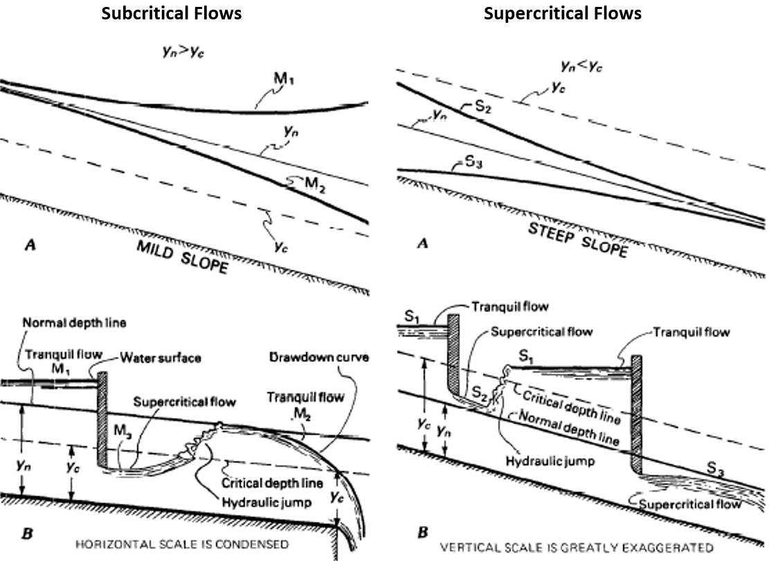
Figure 5.9: Types of flow profiles on mild and steep slopes
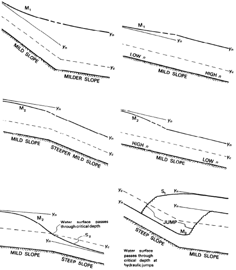
Figure 5.10: Types of flow profiles with changes in slope or roughness
Typically, for supercritical flow the calculations start at an upstream cross section and move downstream. For subcritical flow calculations proceed upstream. However, for the direct step method, a negative result will indicate upstream, and a positive result indicates downstream.
If the water surface passes through critical depth (from supercritical to subcritical or the reverse) it is no longer gradually varied flow and the methods in this section do not apply. This can happen at abrupt changes in channel slope or roughness, or channel transitions.
5.7.1 The direct step method
The direct step method looks at two cross sections in a channel where depths, \(y_1\) and \(y_2\) are defined.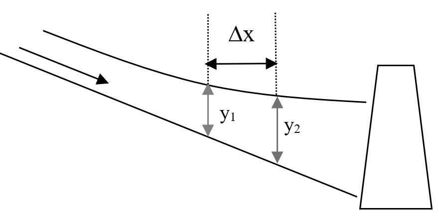
Figure 5.11: A gradually varied flow example.
The distance between these two cross-sections, \({\Delta}X\), is calculated using Equation (5.25) \[\begin{equation} {\Delta}X=\frac{E_1-E_2}{\overline{S}-S_0} \tag{5.25} \end{equation}\] Where E is the specific energy from Equation (5.18), \(S_0\) is the slope of the channel bed, and \(S\) is the slope of the energy grade line. \(\overline{S}\) is the average of the S values at each cross section calculated using the Manning equation, Equation (5.2) solved for slope, as in Equation (5.26). \[\begin{equation} S=\frac{n^2\,V^2}{C^2\,R^{\frac{4}{3}}} \tag{5.26} \end{equation}\]
Example 5.6 demonstrates this.
Example 5.6 Water flows at 10 m3/s in a trapezoidal channel with n=0.015, bottom width 3 m, side slope of 2:1 (H:V) and longitudinal slope 0.0009 (0.09%). At the location of a USGS stream gage the flow depth is 1.4 m. Use the direct step method to find the distance to the point where the depth is 1.2 m and determine whether it is upstream or downstream.
Begin by setting up a function to calculate the Manning slope and setting up the input data.
#function to calculate Manning slope
slope_f <- function(V,n,R,C) {
  return(V^2*n^2/(C^2*R^(4./3.)))
}
#Now set up input data ##################################
#input Flow
Q=10.0
#input depths:
y1 <- 1.4 #starting depth
y2 <- 1.2 #final depth
#Define the number of steps into which the difference in y will be broken
nsteps <- 2

#channel geometry:
bottom_width <- 3
side_slope <- 2         #side slope is H:V. Use zero for rectangular
manning_n <- 0.015
long_slope <- 0.0009
units <- "SI"           #"SI" or "Eng"
if (units == "SI") {
  C <- 1                #Manning constant: 1 for SI, 1.49 for US units
  g <- 9.81
} else {                #"Eng" means English, or US system
  C <- 1.49
  g <- 32.2
}

#find depth increment for each step, depths at which to solve
depth_incr <- (y2 - y1) / nsteps
depths <- seq(from=y1, to=y2, by=depth_incr)
First check to see if the flow is subcritical or supercritical and find the normal depth. Critical and normal depths can be calculated using the manningt function in the hydraulics package, as in Example 5.2. However, because other functionality of the rivr package is used, these will be calculated using functions from the rivr package.
rivr::critical_depth(Q = Q, yopt = y1, g = g, B = bottom_width , SS = side_slope)
#> [1] 0.8555011
#note using either depth for yopt produces the same answer
rivr::normal_depth(So = long_slope, n = manning_n, Q = Q, yopt = y1, Cm = C, B = bottom_width , SS = side_slope)
#> [1] 1.147137
The normal depth is greater than the critical depth, so the channel has a mild slope. The beginning and ending depths are above normal depth. This indicates the profile type, following Figure 5.9, is M-1, so the flow depth should decrease in depth going upstream. This also verifies that the flow depth between these two points does not pass through critical flow, so is a valid gradually varied flow problem.
For each increment the \({\Delta}X\) value needs to be calculated, and they need to be accumulated to find the total length, L, between the two defined depths.
#loop through each channel segment (step), calculating the length for each segment.
#The channel_geom function from the rivr package is helpful
L <- 0
for ( i in 1:nsteps ) {
  #find hydraulic geometry, E and Sf at first depth
  xc1 <- rivr::channel_geom(y=depths[i], B=bottom_width, SS=side_slope)
  V1 <- Q/xc1[['A']]
  R1 <- xc1[['R']]
  E1 <- depths[i] + V1^2/(2*g)
  Sf1 <- slope_f(V1,manning_n,R1,C)

  #find hydraulic geometry, E and Sf at second depth
  xc2 <- rivr::channel_geom(y=depths[i+1], B=bottom_width, SS=side_slope)
  V2 <- Q/xc2[['A']]
  R2 <- xc2[['R']]
  E2 <- depths[i+1] + V2^2/(2*g)
  Sf2 <- slope_f(V2,manning_n,R2,C)

  Sf_avg <- (Sf1 + Sf2) / 2.0
  dX <- (E1 - E2) / (Sf_avg - long_slope)
  L <- L + dX
}
cat(sprintf("Using %d steps, total distance from depth %.2f to %.2f = %.2f m\n", nsteps, y1, y2, L))
#> Using 2 steps, total distance from depth 1.40 to 1.20 = -491.75 m
Figure 5.12: Variation of number of calculation steps to final calculated distance.
The direct step method is also implemented in the hydraulics package, and can be applied to the same problem as above, as illustrated in Example 5.7.
Example 5.7 Water flows at 10 m3/s in a trapezoidal channel with n=0.015, bottom width 3 m, side slope of 2:1 (H:V) and longitudinal slope 0.0009 (0.09%). At the location of a USGS stream gage the flow depth is 1.4 m. Use the direct step method to find the distance to the point where the depth is 1.2 m and determine whether it is upstream or downstream.
hydraulics::direct_step(So=0.0009, n=0.015, Q=10, y1=1.4, y2=1.2, b=3, m=2, nsteps=2, units="SI")
#> y1=1.400, y2=1.200, yn=1.147, yc=0.855585
#> Profile type  = M1
#> # A tibble: 3 × 7
#>       x     z     y     A       Sf     E    Fr
#>   <dbl> <dbl> <dbl> <dbl>    <dbl> <dbl> <dbl>
#> 1    0  0       1.4  8.12 0.000407  1.48 0.405
#> 2 -192. 0.173   1.3  7.28 0.000548  1.40 0.466
#> 3 -492. 0.443   1.2  6.48 0.000753  1.32 0.541
This produces the same result, and verifies that the water surface profile is type M-1.
5.7.2 Standard step method
The standard step method works similarly to the direct step method, except from one known depth the second depth is determined at a known distance, L. This is a preferred method when the depth at a critical location, such as a bridge, is needed.
The rivr package implements the standard step method in its compute_profile function. To compare it to the direct step method, check the depth at \(y_2\) given the total distance from Example 5.6.
Example 5.8 For the same channel and flow rate as Example 5.6, determine the depth of water at the distance L determined above.
The function requires the distance to be positive, so apply the absolute value to the L value.
dist = abs(L)
ans <- rivr::compute_profile(So = long_slope, n = manning_n, Q = Q, y0 = y1, Cm = C, g = g, B = bottom_width, SS = side_slope, stepdist = dist/nsteps, totaldist = dist)
#Distances along the channel where depths were determined
ans$x
#> [1]    0.0000 -245.8742 -491.7483
#Depths at each distance
ans$y
#> [1] 1.400000 1.277009 1.200592
This shows the distances and depths at each of the steps defined. Consistent with the above, the distances are negative, showing that they are progressing upstream. The results are identical for \(y_2\) using the direct step method.
5.8 Rapidly varied flow (the hydraulic jump)
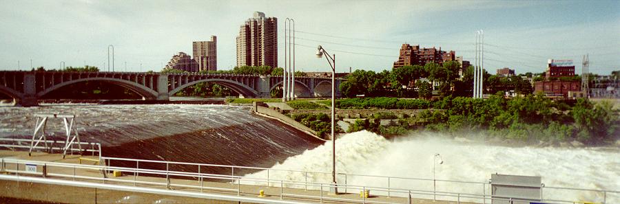
Figure 5.13: A hydraulic jump at St. Anthony Falls, Minnesota.
In the discussion of critical flow in Section 5.5, the concept of alternate depths was introduced, where a given flow rate in a channel with known geometry typically may assume two possible values, one subcritical and one supercritical. For the case of supercritical flow transitioning to subcritical flow, a smooth transition is impossible, so a hydraulic jump occurs. A hydraulic jump always dissipates some of the incoming energy. A hydraulic jump is depicted in Figure 5.14 (Peterka, Alvin J., 1978).
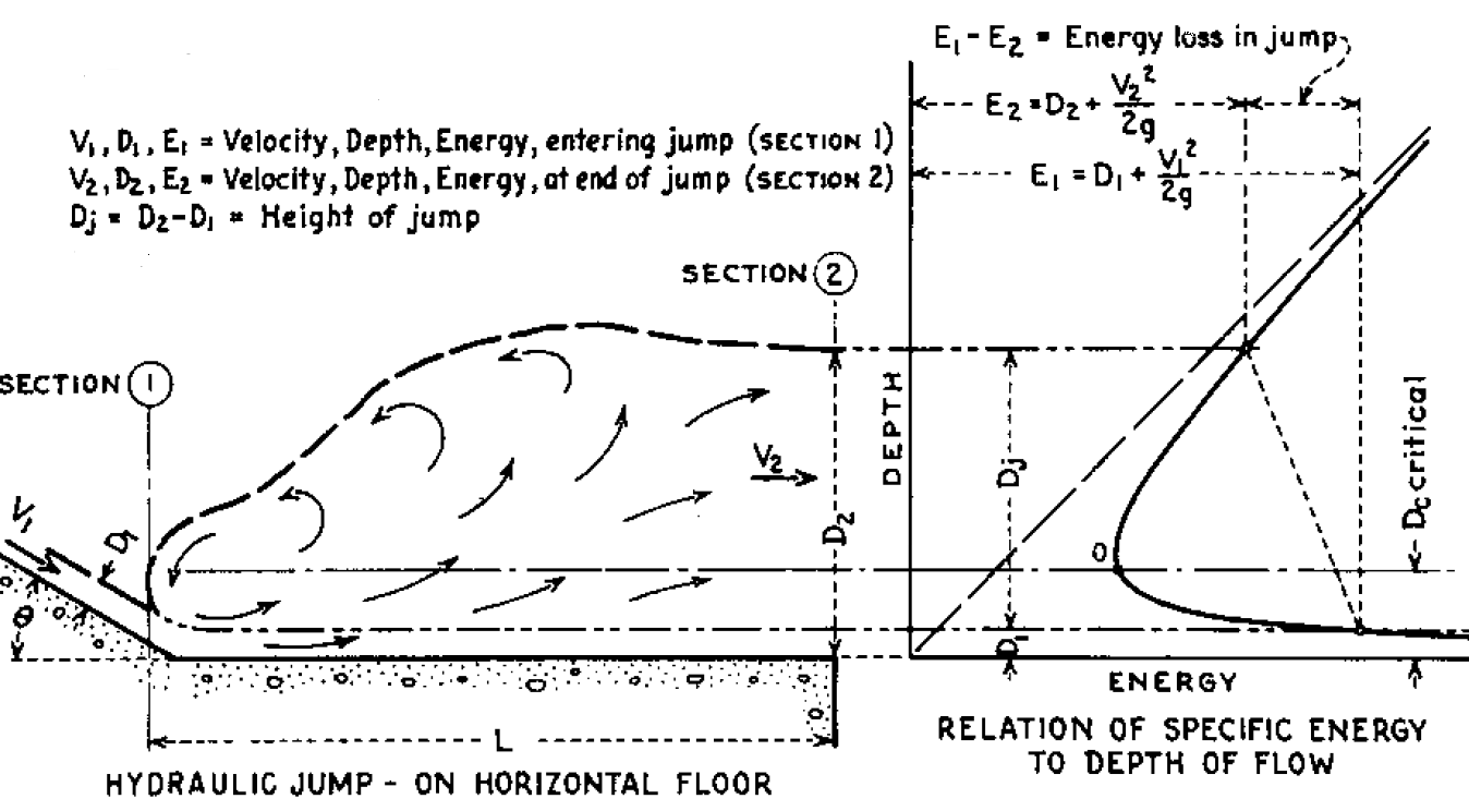
Figure 5.14: A typical hydraulic jump.
5.8.1 Sequent (or conjugate) depths
The two depths on either side of a hydraulic jump are called sequent depths or conjugate depths. The relationship between them can be established using the momentum equation to develop an general expression (for any open channel) for the momentum function, M, as in Equation (5.27). \[\begin{equation} M=Ah_c+\frac{Q^2}{gA} \tag{5.27} \end{equation}\] where \(h_c\) is the distance from the water surface to the centroid of the channel cross-section. For a trapezoidal channel, the momentum equation becomes that described by Equation (5.28). \[\begin{equation} M=\frac{by^2}{2}+\frac{my^3}{3}+\frac{Q^2}{gy\left(b+my\right)} \tag{5.28} \end{equation}\]
For the case of a rectangular channel, setting m=0 and setting the Momentum function for two sequent depths, y1 ans y2 equal, produces the relationship in Equation (5.29). \[\begin{equation} \frac{y_2}{y_1}=\frac{1}{2}\left(-1+\sqrt{1+8Fr_1^2}\right) or \frac{y_1}{y_2}=\frac{1}{2}\left(-1+\sqrt{1+8Fr_2^2}\right) \tag{5.29} \end{equation}\] where Frn is the Froude Number [Equation (5.1)] at section n.
Again, for the case of a rectangular channel, the energy head loss through a hydraulic jump simplifies to Equation (5.30). \[\begin{equation} h_l=\frac{\left(y_2-y_1\right)^3}{4y_1y_2} \tag{5.30} \end{equation}\]
Given that the momentum function must be conserved on either side of a hydraulic jump, finding the sequent depth for any known depth becomes straightforward for trapezoidal shapes. Setting M1 = M2 in Equation (5.28) allows the use of a solver, as in Example 5.9.
Example 5.9 A trapezoidal channel with a bottom width of 0.5 m and a side slope of 1:1 carries a flow of 0.2 m3/s. The depth on one side of a hydraulic jump is 0.1 m. Find the sequent depth, the energy head loss, and the power dissipation in Watts.
flow <- 0.2
ans <- hydraulics::sequent_depth(Q=flow,b=0.5,y=0.1,m=1,units = "SI", ret_units = TRUE)
#print output of function
as.data.frame(ans)
#>                  ans
#> y            0.1 [m]
#> y_seq  0.3941009 [m]
#> yc      0.217704 [m]
#> Fr      3.635731 [1]
#> Fr_seq 0.3465538 [1]
#> E       0.666509 [m]
#> E_seq  0.4105265 [m]
#Find energy head loss
hl <- abs(ans$E - ans$E_seq)
hl
#> 0.2559825 [m]
#Express this as a power loss
gamma <- hydraulics::specwt(units = "SI")
P <- gamma*flow*hl
cat(sprintf("Power loss = %.1f Watts\n",P))
#> Power loss = 501.4 Watts
The energy loss across hydraulic jumps varies with the Froude number of the incoming flow, as shown in depicted in Figure 5.15 (Peterka, Alvin J., 1978).
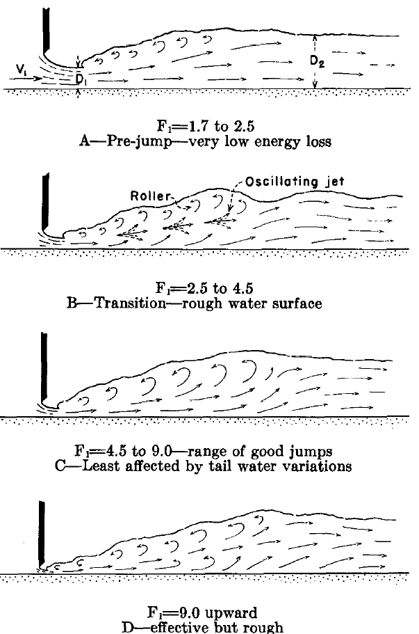
Figure 5.15: Types of hydraulic jumps.
5.8.2 Location of a hydraulic jump
In hydraulic infrastructure where hydraulic jumps will occur there are usually engineered features, such as baffles or basins, to force a hydraulic jump to occur in specific locations, to protect downstream waterways from the turbulent effects of an uncontrolled hydraulic jump. In the absence of engineered features to cause a jump, the location of a hydraulic jump can be determined using the concepts of Sections 5.7 and 5.8.
Example 5.10 demonstrates the determination of the location of a hydraulic jump when normal flow conditions exist at some distance upstream and downstream of the jump.
Example 5.10 A rectangular (a trapezoid with side slope, m=0) concrete channel with a bottom width of 3 m carries a flow of 8 m3/s. The upstream channel slopes steeply at So=0.018 and discharges onto a mild slope of So=0.0015. Determine the height of the jump and its location.
First find the normal depth on each slope, and the critical depth for the channel.
yn1 <- hydraulics::manningt(Q = 8, n = 0.013, m = 0, Sf = 0.018, b = 3, units = "SI")$y
yn2 <- hydraulics::manningt(Q = 8, n = 0.013, m = 0, Sf = 0.0015, b = 3, units = "SI")$y
yc <- hydraulics::manningt(Q = 8, n = 0.013, m = 0, Sf = 0.0015, b = 3, units = "SI")$yc
cat(sprintf("yn1 = %.3f m, yn2 = %.3f m, yc = %.3f m\n", yn1, yn2, yc))
#> yn1 = 0.498 m, yn2 = 1.180 m, yc = 0.898 m
Recall that the calculation of yc only depends on flow and channel geometry (Q, b, m), so the values of n and Sf can be arbitrary for that command. These results confirm that flow is supercritical upstream and subcritical downstream, so a hydraulic jump will occur.
The hydraulic jump will either begin at yn1 (and jump to the sequent depth for yn1) or end at yn2 (beginning at the sequent depth for yn2). The possibilities are shown in Figure 5.9 in the lower right panel. First check the two sequent depths.
yn1_seq <- hydraulics::sequent_depth(Q = 8, b = 3, y=yn1, m = 0, units = "SI")$y_seq
yn2_seq <- hydraulics::sequent_depth(Q = 8, b = 3, y=yn2, m = 0, units = "SI")$y_seq
cat(sprintf("yn1_seq = %.3f m, yn2_seq = %.3f m\n", yn1_seq, yn2_seq))
#> yn1_seq = 1.476 m, yn2_seq = 0.666 m
This confirms that if the jump began at yn1 (on the steep slope) it would need to jump a level below yn2, with an S-1 curve providing the gradual increase in depth to yn2. Since yn1_seq exceeds yn2, this is not possible. That can be verified using the direct_step function to show the distance from yn1_seq to yn2 would need to be upstream (negative x values in the result), which cannot occur for this case. This means the alternate case must exist, with an M-3 profile raising yn1 to yn2_seq at which point the jump occurs. The direct step method can find this distance along the channel.
hydraulics::direct_step(So=0.0015, n=0.013, Q=8, y1=yn1, y2=yn2_seq, b=3, m=0, nsteps=2, units="SI")
#> # A tibble: 3 × 7
#>       x       z     y     A      Sf     E    Fr
#>   <dbl>   <dbl> <dbl> <dbl>   <dbl> <dbl> <dbl>
#> 1   0    0      0.498  1.49 0.0180   1.96  2.42
#> 2  23.4 -0.0350 0.582  1.75 0.0113   1.65  1.92
#> 3  44.6 -0.0669 0.666  2.00 0.00761  1.48  1.57
The number of calculation steps (nsteps) can be increased for greater precision, but 2 steps is adequate here.