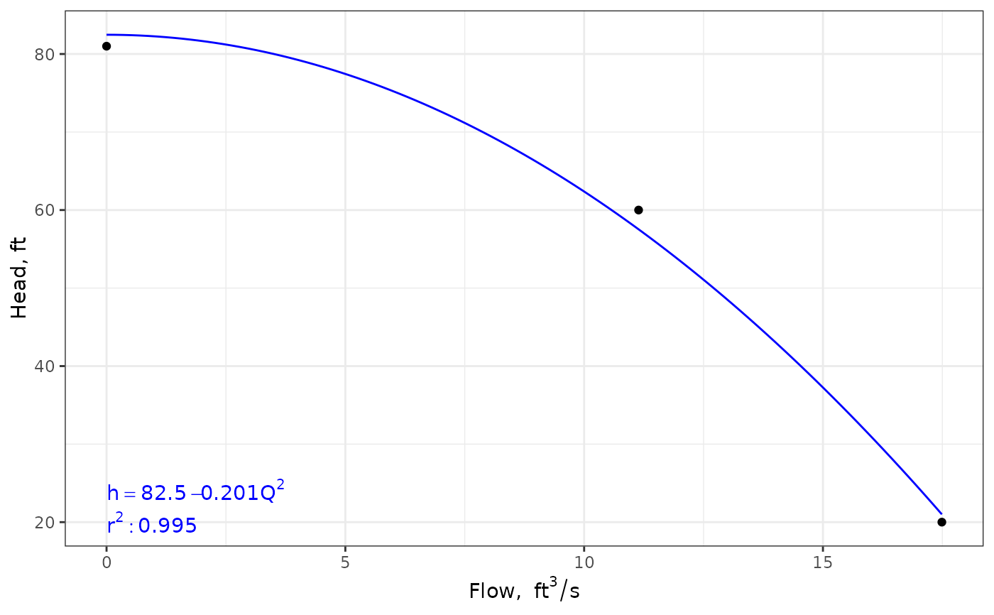
Fits a polynomial curve to three or more points from a pump characteristic curve to be used in solving for an operating point of the pump in a piping system.

Fits a polynomial curve to three or more points from a pump characteristic curve. This allows solving for an operating point of the pump in a piping system. A portion of this is based on https://github.com/PhDMeiwp/basicTrendline/blob/master/R/trendline.R

Usage

pumpcurve(Q = NULL, h = NULL, eq = "poly1", units = c("SI", "Eng"))

Arguments

Q

Numeric vector of flow rates for selected points on the pump curve [\(m^3 s^{-1}\) or \(ft^3 s^{-1}\)]

h

Numeric vector of heads for selected points on the pump curve [\(m\) or \(ft\)]

eq

Character vector identifying the for of equation to fit (see details)

units

character vector that contains the system of units [options are SI for International System of Units and Eng for English (US customary) units.

Value

Returns an object of class pumpcurve consisting of a list including:

• curve - a function defining the curve that is fit to the data

• eqn - a character vector of the equation for the curve

• r2 - the coefficient of determination for the curve fit, \(R^2\)

• p - a plot object of the fit curve

• units - the units system passed to the function

Details

The form of the equation fit to the input points may be one of the following, as determined by the eq input parameter.

eq	equation form
poly1	\(h = a + {b}{Q} + {c}{Q}^2\)
poly2	\(h = a + {c}{Q}^2\)
poly3	\(h = h_{shutoff} + {c}{Q}^2\)

where \(h_{shutoff}\) is the head on the pump curve associated with \(Q=0\). The shutoff head at \(Q=0\) should be included in the input vectors if the poly3 equation form is to be used.

Author

Ed Maurer

Examples

#Input in Eng units - use \code{units} package for easy unit conversion
qgpm <- units::set_units(c(0, 5000, 7850), gallons/minute)
qcfs <- units::set_units(qgpm, ft^3/s)
hft <- c(81, 60, 20) #units are already in ft so setting units is optional
pumpcurve(Q = qcfs, h = hft, eq = "poly2", units = "Eng")
#> $curve
#> function (x) 
#> coef(hqfit)[1] + x^2 * coef(hqfit)[2]
#> <bytecode: 0x5601ba7c1260>
#> <environment: 0x5601ba7bf900>
#> 
#> $eqn
#> [1] "h == 82.5 - 0.201*Q^2"
#> 
#> $r2
#> [1] 0.995
#> 
#> $p

#> 
#> $units
#> [1] "Eng"
#> 
#> attr(,"class")
#> [1] "pumpcurve"